Proximal Policy Optimization

Introduction

In the previous post, we discussed the Trust Region Policy Optimization (TRPO) method for solving the full Reinforcement Learning problem. TRPO builds upon the Natural Policy Gradient approach, with a series of approximations for solving the second-order optimization problem. Despite all the theoretical guarantees that TRPO gives, it does not work very well in practice on some problems. There can be two reasons for this -

1. The errors introduced due to approximations magnify and, in turn, lead to divergence of the policy parameters.

2. Even if the policy converges, it is likely to be stuck in a local optimum. This is because TRPO makes an update only when it is guaranteed an improvement. Once a policy converges to a local optimum, since the updates introduce no more noise in the parameters, there is no chance for the parameters to slip off a local optimum to move towards the global optimum. As a result, it leads to a sub-optimal policy.

So how do we overcome these two demerits?

When the Lion takes two steps back, it does so to pounce not to flee!! xD

This quote gives a perfect analogy to our case. We need to do exactly like the Lion!

So if we are introducing errors due to the approximation of the second-order optimization problem, go back to our old friendly first-order optimization methods, which are computationally easier to deal with. Also, it is fine to sometimes tweak the policy parameters such that it does not lead to improvement. That is, it is not necessary that we guarantee monotonic improvement at every single update. This means that we should not be greedy about the short-term goal and instead, focus more on the long-term goals of achieving convergence to the globally optimal policy.

This is exactly what Proximal Policy Optimization (PPO) does. Its simplicity and efficiency at the same time have made it the default algorithm for most of the applications in RL.

PPO is an on-policy algorithm that builds a stochastic policy by tweaking the policy parameters, which are parameterized by a function approximator like Neural Net. It can be used in infinite state-space environments with continuous as well as discrete action-spaces.

Exploration v/s Exploitation

PPO balances between Exploration and Exploitation like other on-policy methods. Since it is on-policy, it samples behavior from the same policy it optimizes. Initially, the exploration rate is higher as compared to the exploitation so that it can explore the state space. Eventually, the policy focuses more on exploiting the rewards already found. This, however, can lead to the policy converging to a sub-optimal policy, which is a downside of all policy-based methods.

I hope that you have gone through my previous post on TRPO. I assume that you have the necessary knowledge to understand the Maths behind the equation below from my previous article. I will start building the idea and intuition behind PPO from the following equation:

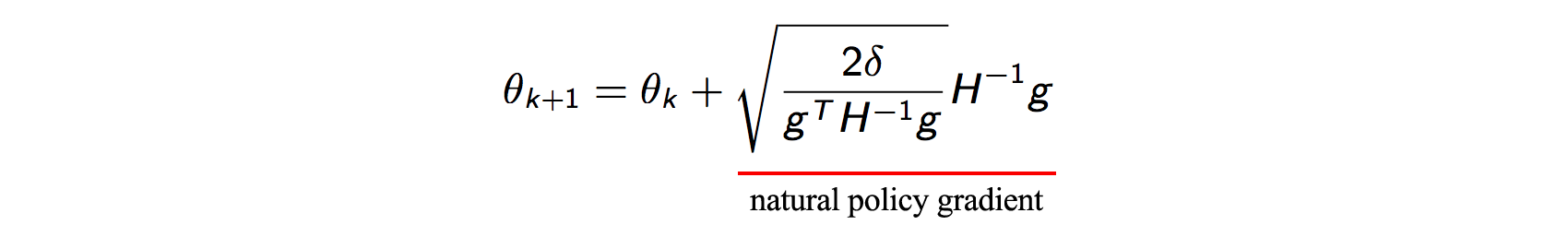
After all the math in the TRPO post, we arrive at this policy parameter update to limit the policy changes and to ensure monotonic policy improvement. So what are the challenges associated with solving this optimization update?

In TRPO, the inverse of the Hessian $H$ is approximated using the Conjugate Gradient algorithm with the help of a few Hessian-vector products, thus avoiding the expensive computation. However, we still need the Hessian $H$. To avoid computing the second-derivatives, we use the Fisher Information Matrix (FIM) which is equal to the following -

Though not obvious, F can be interpreted as the negative expected Hessian of our log-likelihood model. Hence from now on, I will be using $F$ and $H$ interchangeably in this post.

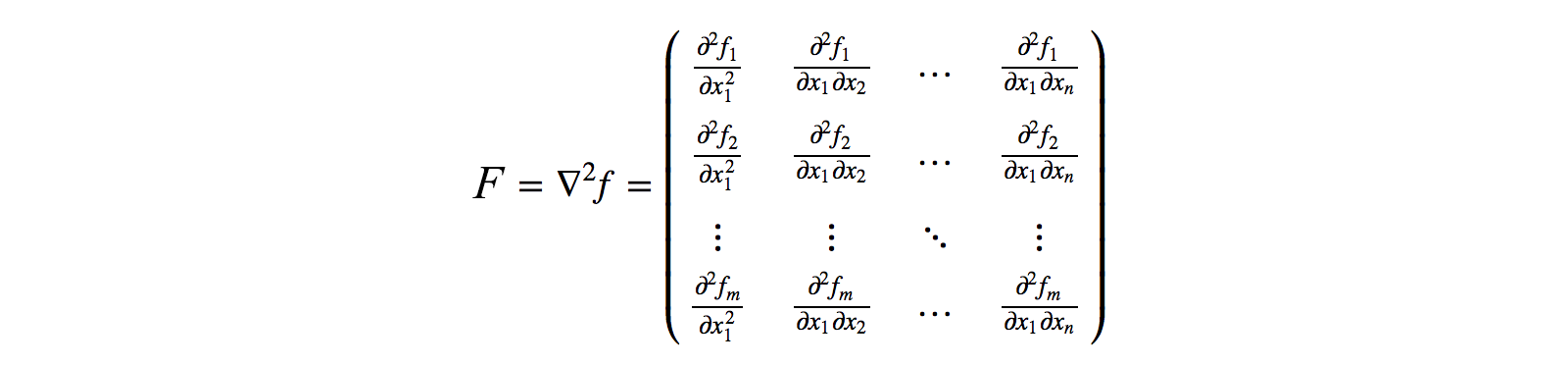
$F$ can be seen basically as a matrix of all the second-order derivatives (with respect to $\theta$) of the function, which in our case, is the $\log$ of the parameterized policy.

F can be computed as the expected value of the product of the log-likelihood function as illustrated before.

As we know, calculating the matrix $F$ and its inverse is computationally very expensive, especially for the non-linear policies parameterized by Deep Neural Nets. So, we approximate the inverse by converting the problem to a quadratic optimization, as shown in the above image. However, we still need to compute the matrix $F$, which is shown above. Hence we can proceed with either of these two -

1. Build more sophisticated methods to approximate these second-order derivative matrices to lower the computational complexity.

2. Narrow the gap between the first and second-order optimization methods by adding some soft constraints (to make sure that the old and the new policies are not very different from each other and policy improvement over time, though not strictly monotonic) to the first-order optimization.

We did exactly the first way in TRPO. However, PPO follows an approach similar to the second method. Yes, PPO is a first-order optimization method!!

There are two versions of PPO. Let us look at them one by one.

PPO with adavptive KL-Penalty

This approach is similar to what we do in TRPO, except that we optimize using Stochastic Gradient Ascent, a first-order optimization method, and vary the KL-penalty according to our requirement.

Here, our optimization objective looks like the above equation. Using the Lagrange Duality, the PPO objective with the adaptive KL penalty can be shown to be equivalent to the constrained optimization problem in TRPO. This basically penalizes the advantage when the policies are different; that is, the KL divergence is high.

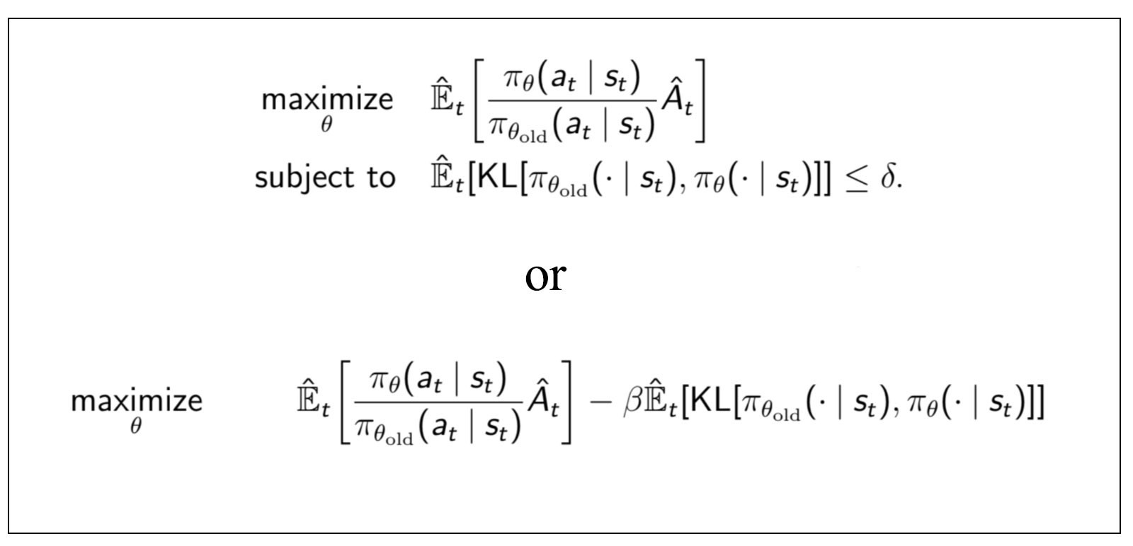
Note that the hyperparameter $\delta$ (radius of the trust region) and $\beta$ (the adaptive penalty) are inversely related.

As we see in the penalty form of the objective, choosing a constant value for the hyperparameter $\beta$ can lead to bad or disastrous policy (please refer my TRPO post to get an idea of a bad policy). So we can dynamically vary $\beta$ so that it adapts to meet our requirements -

1. When the KL divergence between the old and the new policies gets higher than a threshold value, then we can shrink the trust-region $\delta$, which is equivalent to increasing $\beta$. We do this to make sure that both the policies do not differ much, and we do not take large steps.

2. The reverse holds when the KL divergence falls below a certain threshold. We increase the radius of the trust region $\delta$, thereby decreasing $\beta$. We do this to speed-up the learning process and to relax the constraints a bit.

Image Source

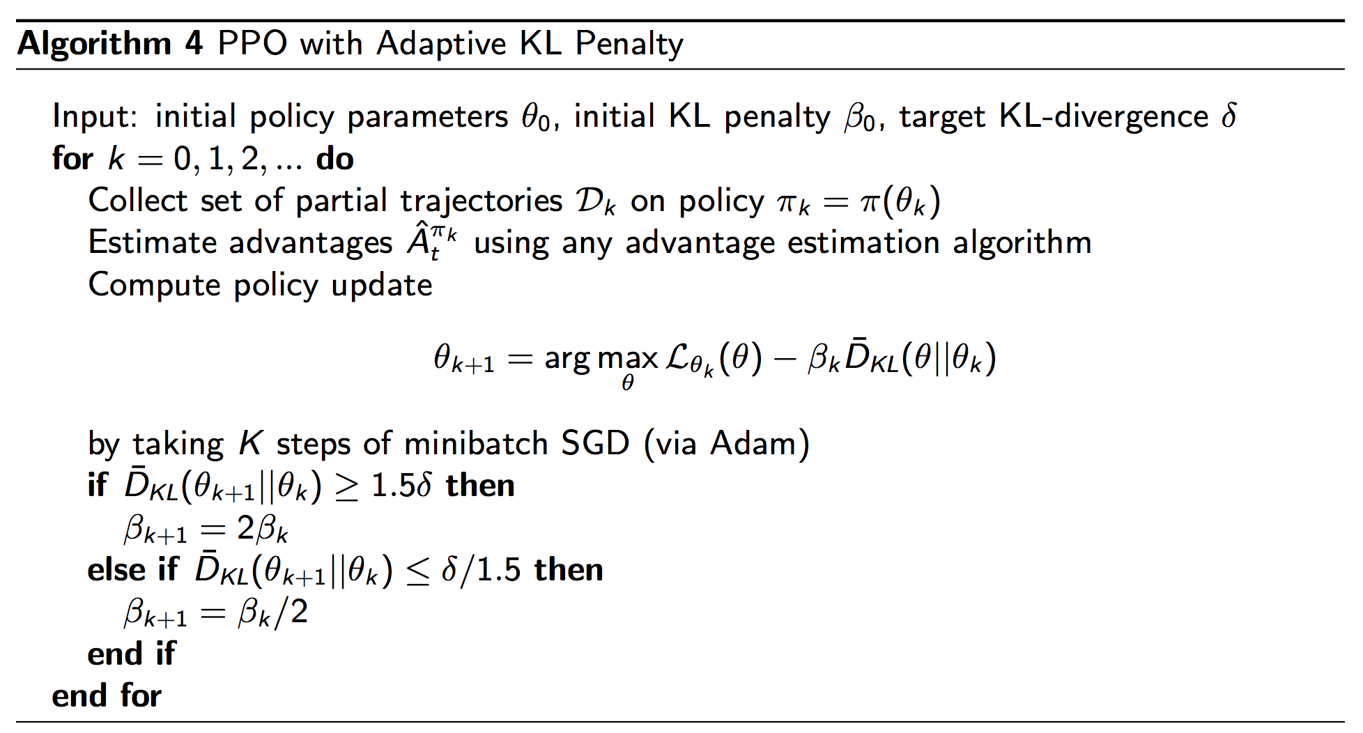
The figure above shows the pseudo-code for PPO with Adaptive KL Penalty. Note the changes in $\beta$.

Doing this gets us the best of both the worlds. We get the speed close to first-order optimization methods as well as performance close to TRPO. But can we do better?

PPO with Clipped objective

With PPO, we are not guaranteed to find monotonic policy improvement at each step; however, adapting $\beta$ accordingly, tends to work well in practice for improving convergence. In the clipped version of PPO, we remove the KL-divergence term and instead use clipping to make sure that the new policy does not go very far from the old one, despite incentives for better improvement. We modify the objective function as follows -

\[L(s,a,\theta_k,\theta) = \min\left(\frac{\pi_{\theta}(a|s)}{\pi_{\theta_k}(a|s)} A^{\pi_{\theta_k}}(s,a), \text{clip}\left(\frac{\pi_{\theta}(a|s)}{\pi_{\theta_k}(a|s)}, 1 - \epsilon, 1+\epsilon \right) A^{\pi_{\theta_k}}(s,a) \right)\]

Here $\pi(\theta)$ is the old policy and $\pi(\theta_k)$ is the new one. We use the Importance Sampling technique to sample trajectories from the old policy while updating the new one. This improves sample efficiency.

At first sight, it may be a bit hard to decode what this new objective says. Let me break it down into two parts -

1. When the Advantage function is non-negative

\[L(s,a,\theta_k,\theta) = \min\left(\frac{\pi_{\theta}(a|s)}{\pi_{\theta_k}(a|s)}, (1+\epsilon)\right) A^{\pi_{\theta_k}}(s,a)\]

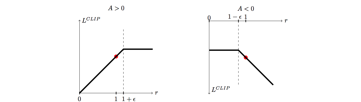
The Advantage function is nothing but the return (Monte-Carlo or TD-return or the Q-function) from the current state-action pair minus the baseline (chosen such that it does not depend on the policy parameters). When the advantage is $0$, we are in a neutral position. Considering the other possibility, if the advantage is positive, it means that taking action $a$ in the state $s$ is more likely to improve the performance. Hence, we should increase the probability of taking action $a$ in the state $s$. However, increasing does not mean we can do it without an upper limit.

$\epsilon$ in the above equation takes a small value between $0$ and $1$ ($0.2$ in the PPO paper). $\min$ in the above equation means that the correction ratio will be clipped as soon as it passes the upper limit $(1+\epsilon)$. This will ensure a limited increment in the objective, even if a higher ratio leads to more improvement.

You can view this clipping similar to what we do in trust-region. We find the most optimal point in the trust-region and use it as our next estimate of the policy while ignoring any other point outside the trust-region, even if we might improve more. We do this because our bets are off in the space outside the trust-region.

1. When the Advantage function is negative

\[L(s,a,\theta_k,\theta) = \max\left(\frac{\pi_{\theta}(a|s)}{\pi_{\theta_k}(a|s)}, (1 - \epsilon)\right) A^{\pi_{\theta_k}}(s,a)\]

When the advantage function is a negative value, it means that action $a$ is not favorable to take in the state $s$. Hence, we should decrease the probability of the same. We do this by imposing a $\max$ constraint this time. It means that even though decreasing the probability ratio below $(1-\epsilon)$ would result in better performance, we do not do so, to make sure that the policies do not diverge much.

By seeing the above two versions of the objective function under different conditions, we understand the clipped version of PPO. This clipping makes sure that the new policy does not benefit by going too far from the old policy. Imposing these two constraints helps us achieve the same results as KL-divergence and sometimes even better. Following is a visualization of the objective function -

Image Source

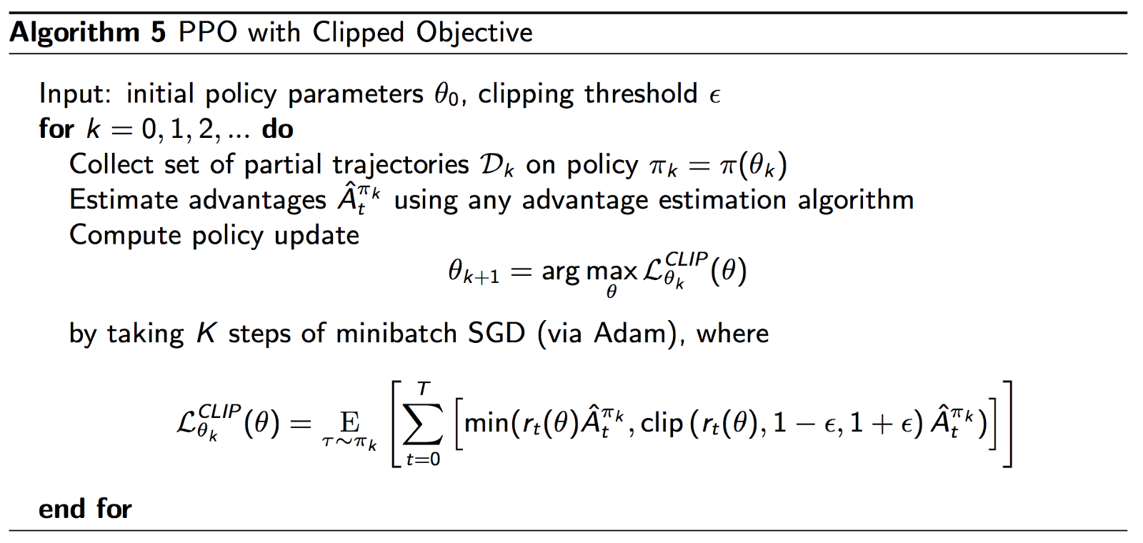
Finally, we put together all the pieces to form the PPO algorithm with Clipped objective -

Image Source

End thoughts

What we saw in this post is a great example of how well SIMPLICITY rules in Machine Learning. PPO might not give a monotonic improvement of the policy in each update, but ensures overall improvement in the end for most of the time. We can guess the reason for this. As we all know, Machine Learning, whether it may be supervised, unsupervised or reinforcement learning is all about Applied Optimization. So for convergence in practice, it is good to behave like the Lion :P and sacrifice the current local benefits in order to achieve more important goals in the future (being quite non-technical here). However, we need to do this trick carefully, ensuring minimum losses, as we do by imposing certain soft constraints on $\beta$ in the PPO KL-Penalty version and by clipping in the PPO Clipped version.

So PPO gives pretty good results on standard benchmarks like Atari and other continuous control environments like in OpenAI Gym. However, despite all of it, this is just a beginning as the achievements of the RL and AI community for solving even the most simple real-world robotics problems like making a robot pick a glass of water or to do the dishes, are not much exciting. No worries about it. There’s always room for improvement and indeed we’re just a few break-through papers away for achieving convincing results! :)