Trust Region Policy Optimization

In this article, we will look at the Trust Region Policy Optimization (TRPO) algorithm, a direct policy-based method for finding the optimal behavior in Reinforcement Learning problems.

So what is TRPO??

TRPO is an on-policy method belonging to the class of Policy Gradient (PG) methods that optimize a stochastic policy directly by improving it by tweaking the policy parameters $\theta$. The policy can be parameterized by any of the function approximators like Neural Networks, Decision Trees, etc. However, Neural Nets are the most popular class of models used to represent a policy. TRPO can be used in infinite state-space environments with continuous as well as discrete action-spaces.

Exploration v/s Exploitation

TRPO balances Exploration and Exploitation, similar to other PG methods. Since it follows an on-policy approach, it explores naturally by sampling actions according to the latest version of the stochastic policy. The degree of randomness depends both on the training procedure and the initial conditions. Eventually, the policy becomes less exploratory as the training time increases since it focuses more on exploiting the rewards already found. Like other PG methods, TRPO has a disadvantage of being stuck in a Local Optima. This is one of the downsides of PG methods over Value-Based methods.

But why do we need a TRPO approach for PG methods?

TRPO is a variant of PG methods for policy optimization. One might want to contrast this algorithm with the traditional REINFORCE or online Actor-Critic (AC) approach. So the question that arises is, what are the problems associated with Vanilla PG (VPG) or Actor-Critic (AC) methods and how does TRPO overcome these? To seek the answer, we have to dive deeper into the nitty-gritty details of Policy gradients. Let’s go!

Important

Note: From now, when I refer to PG methods, I mean the Vanilla PG (REINFORCE) and AC approach.

• If we see the update rule for the PG methods, it is based on Gradient Ascent, which is nothing but a first-order optimization. So we use first-order derivatives (tangent at that point) and approximate the surface to be flat. If the surface has a high curvature, then we can make horrible moves, and this is the case with PG methods.

• Unlike Supervised Learning, the input data that we use to make the updates is non-stationary in RL. This is because we sample the states and the actions (data) by experiencing the latest version of our policy. When we update, the observation and reward distributions change. This is one of the major reasons for the lack of stability in optimization methods in RL. From this, we also conclude that it is not preferable to have a fixed step-size (learning rate) for optimization in RL. The PG methods use a fixed learning rate, which is not sensitive to the shape and curvature of the reward function.

  • We can view the problem associated with an example. Suppose at some point, the reward function is more or less flat. So it makes sense to use a learning rate larger than the average for a good learning speed. However, one bad move (during the update) may result in taking a large step to the steep regions where a large learning rate may result in disastrous policy updates. So the learning rate needs to be sensitive to the surface that we are optimizing (reward function). Now, let me explain what “disastrous” meant. So a step too far in the steep regions on the surface might result in bad policy for which the reward we get is lower than the average. The next batch of states and actions in the following update iteration will be sampled from this bad policy. In turn, this sequential process will continue, and it would be very difficult to recover, and will eventually lead to a collapse in the performance.

  • Note that I am being highly non-technical for this example in highlighting the consequences of having fixed learning-rates and non-optimal policies. Nevertheless, this instance was just to give an intuition of what is happening to the policy parameters in the high-dimensional space during optimization process.

• One clear conclusion that can be made from the above point is that we need to limit the policy changes, and if possible, also make sure that the policy changes for good (Fun Fact: TRPO does exactly this for us!!). So how about adding some threshold to the change in policy parameter $\theta$. PG methods can achieve this by keeping the new and old policy parameters close to each other in the parameter space. However, seemingly small changes in the parameter space could result in large changes in the policy space. So we cannot make sure that a small update in the parameters would result in something similar in the policy. Our main objective, however, is to limit the policy changes. So we need to find some way to translate the change in the Policy Space $\pi(\theta)$ to the model Parameter Space $\theta$.

• One more downfall associated with PG methods is Sample Efficiency. For PG methods, we sample a whole trajectory for a single policy parameter update. We can have thousands of time-steps in a trajectory, or even more, depending on the environment, and for obtaining an optimal policy, we need to make numerous updates depending upon the training procedure and initial parameter values. This, as we can see, is quite a sample inefficient. But why don’t we make an update per time-step? The answer to this question is in the very requirement for function approximators for handling high-dimensional RL problems. Tabular RL methods, as we all know, are not suited for problems with large state and action spaces. But have you ever wondered how only a finite number of parameters could approximate an infinite number of state-action values with decent accuracy? This is because the states in such continuous environments are closely related to each other. For some visualization, imagine the environment to be a large maze. Usually, the value of the state the agent is currently in is not very different from the value of a state a few centimeters away from it. Hence the states are closely related.

  • Now having justified this, let us come back to our main question about updating per time-step. If we make updates in each time-step, it will result in similar updates multiple times at similar spots on the surface (since the reward for similar spots is not very different). This makes the training unstable and sensitive as changes reinforce and magnify. Hence, we need to make one update per trajectory to ensure the stability and convergence of the policy. You can also view this idea by contrasting Stochastic Gradient Descent (SGD) and Mini-Batch Gradient Descent (MBGD). These two, as we know, are first-order optimization methods, and are standard for optimizing any Supervised Learning problem. The difference is that the former makes one update per training example, and the latter calculates the loss for some arbitrary N number of updates and then sums it and uses it for making an update. In general, even in supervised learning, MBGD tends to be more stable than SGD. It requires a bit more computation but gives better results.

So the four points highlighted above tell us the demerits associated with normal PG methods (VPG and AC without experience replay) and the need for a better optimization technique. Basically, we want to ensure two things:

1. We need to limit the policy changes so that the new and the old policies don’t differ much.
2. At the same time, we should ensure that any change in policy guarantees a monotonic improvement in rewards.

TRPO ensures this for us!! Let us see how

Minorize-Maximization Algorithm

The Minorize-Maximization (MM) algorithm gives us the theoretical guarantees that the updates always result in improving the expected rewards. A simple one line explanation of this algorithm is that it iteratively maximizes a simpler lower bound function (lower bound with respect to the actual reward function), approximating the reward function locally.

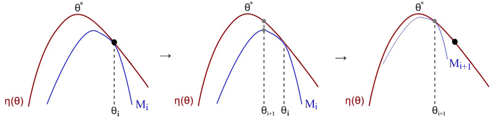
So in this algorithm, we start with an initial policy guess $\pi(\theta_i)$. $\theta_i$ is the policy parameter vector for it at the $i^{th}$ iteration. We find a lower bound function $M_i$ (blue-colored in the above figure) that approximates the actual reward function $\eta(\theta)$ (red-colored in the above figure) locally near $\theta_i$. We will then find the optimal theta $\theta_{i+1}$ for this lower bound function $M_i$ and then use it as our next estimate for the policy $\pi(\theta_{i+1})$. We continue this process, and eventually, the policy parameter converges close to the optimal $\theta^{*}$.

One important thing to keep in mind while implementation is that the lower bound function $M$ should be easier to optimize than the actual reward function, otherwise this algorithm would be pointless.

This approach guarantees monotonic policy improvement (at least theoretically). Now, how do we make sure that the new policy is not very different from the old one? Trust Region comes to rescue here.

Trust Region

Here, we have a maximum step-size $\delta$ which is the radius of our trust region. We call this Trust Region because this acts as a threshold for the policy change. So we can trust any change in the policy within this radius and be sure that it does not degrade the performance. We find the optimal point in this region and resume the search from there. By doing this we are imposing a restriction that we are allowed to explore only a certain region in the policy space, even though at times, an incentive for better policy might be available in some distant part of the policy space.

In the figure above, we maximize our lower bound estimate subject to the condition that the change is limited to $\delta$.

An important point to consider here is the learning speed, which might be slow due to this trust region. Since even though we may find a better policy outside the trust region, we would not consider that as are bets are off in that part of policy space. There is a simple solution to this. We can shrink the trust-region when the KL-divergence between the old and new policies gets large in order not to get over-confident and vice-versa for expanding the region.

Importance Sampling

Importance Sampling(IS) is a tool for calculating the expectation of some function distribution by taking samples from another distribution. We add a correction ratio term in the expectation for this.

The idea of using IS here is to form an objective function, the gradient of which gives the policy gradient.

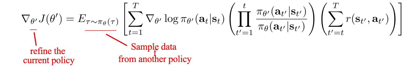
This is the policy gradient. To overcome the sample efficiency problem, we use IS to reuse the data from a slightly old policy while doing updates for the current policy.

$L_{PG}$ is the objective function for our PG as its derivative with respect to $\theta$ gives PG. We can form a Surrogate Advantage function using IS as shown in the above figure, and differentiating it with respect to $\theta$ will result in the same gradient. We can see this Surrogate Advantage as a measure of how the current policy performs relative to the old one using the data from the old policy. It finds the advantage function for the current policy with samples from the old policy.

It is important to note that if we calculate the variance of the Surrogate advantage, it has the term $\pi(\theta_{curr})/\pi(\theta_{old})$ in it. Hence, if the new policy is very different, this ratio will be high, and it’ll explode the variance. This also means that we cannot use the old samples for a very long time. We have to resample after say every 4-5 iterations.

Now we have all the ingredients to jump into TRPO!!

The $\delta$ parameter for the trust region is left as a hyperparameter for us to tweak. However, we need to find a lower bound function $M$ to guarantee monotonic policy improvement. The actual TRPO paper gives detailed proof for this -

I am not going into the details of the proof in this article, but it can be referenced using the results from the paper.

In the LHS, we redefine the objective function as the difference between the reward function of the two policies. This does not affect the optimization problem as the latter term in LHS $J(\pi)$ is constant.

In the RHS, the first term is the Surrogate advantage that we talked about in IS, and the second is the KL-divergence, which measures the difference between two probability distributions.

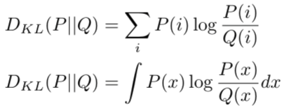
Note that KL-divergence does not measure the distance between the two probability distributions. This is because it is not symmetric and hence cannot be a measure of distance. These two probability distributions will be the two parameterized policies.

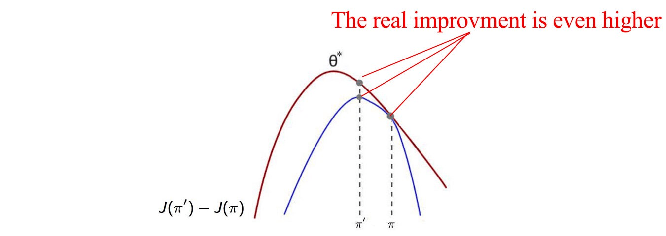
An important note here is that this inequality gives us a concrete proof of the monotonic improvement. This is because, at $\pi$ = $\pi^{\prime}$, the LHS is $0$ and both the terms in the RHS are also $0$. So equality is satisfied. Now since the RHS is a lower bound, the LHS is always greater than or equal to $0$, which means that the new policy is always better than the old. We can, in fact, give a better guarantee that the real improvement in the policy is even higher than it is in the function $M$ as shown in the following figure -

Defining the Optimization problem

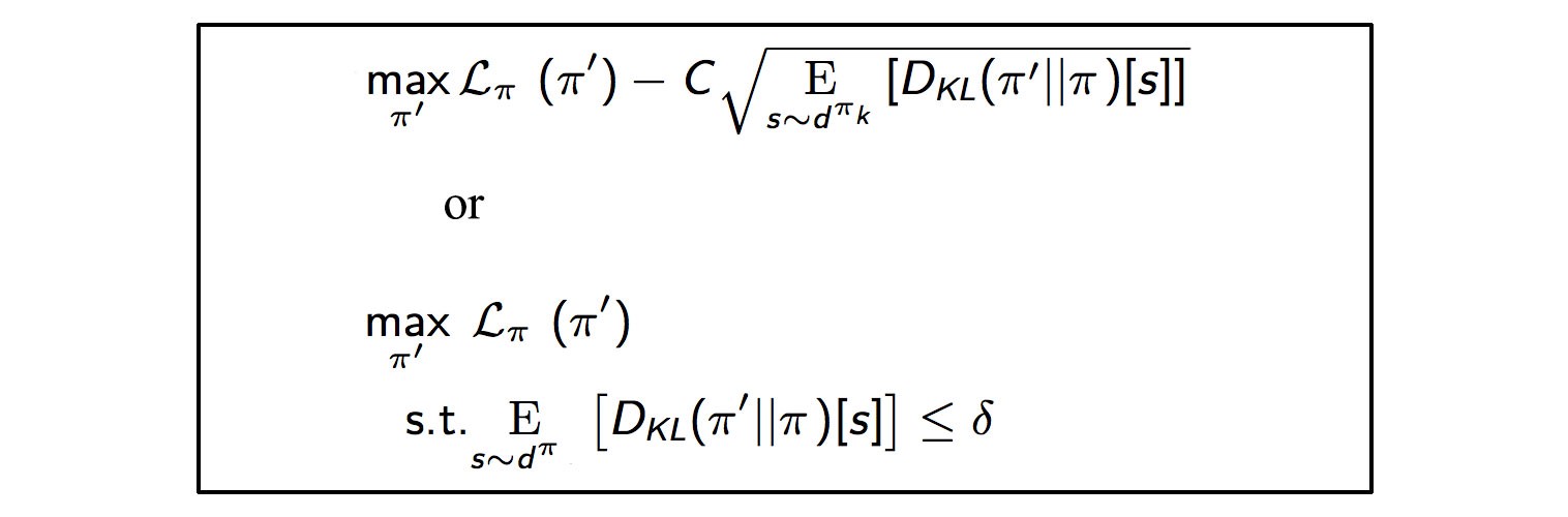
Now we have two versions of the optimization problem. The first is the Penalized version, where we subtract the KL-divergence term scaled by a factor $C$. The second is a Constrained problem with a $\delta$ constraint representing the trust region. $C$ and $\delta$ as we can see are inversely related. Both forms are equivalent according to the Lagrange duality. Theoretically, both arrive at the same solution, but in practice, $\delta$ is easier to tune than $C$. Also, empirical results show that $C$ cannot be a fixed value and needs to be more adaptive. Hence we use the Constrained problem in TRPO.

Fun Fact: These enhancements in the hyperparameter C are made in Proximal Policy Optimization (PPO), another popular algorithm for Reinforcement Learning.

Now how do we solve this Optimization problem?

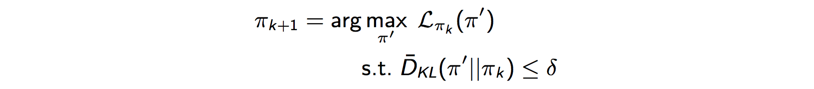
This is our constrained problem. However, solving it accurately would be quite expensive. So we use our old friend from mathematics - the Taylor Polynomial approximation.

This makes sense because we just need to approximate the surrogate advantage locally near our current policy parameter $\theta_k$, and Taylor Polynomials are a very good tool to approximate a function around a particular point in some interval using just polynomial terms, which are a lot easier to deal with as compared to other functions. So we use the Taylor series to expand the Surrogate advantage and the KL-divergence term.

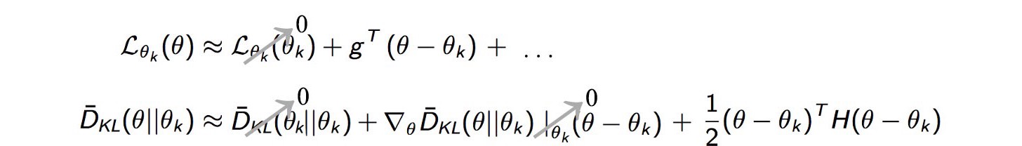
The first term of $L$ is obviously $0$, as for very small policy changes i.e., the state distribution under the two policies are very similar, the difference between the reward functions is close to $L$. Hence for the same policies it is $0$.

Coming to the first term for KL-divergence. It is $0$ because the divergence between the same policy distributions is $0$. The second term is $0$ as if we look at the equation for KL-divergence and differentiate it with respect to $\theta$, it will cancel out the Integral and we will be left with $\log(\pi_{curr}/\pi_{old})$, and putting $\pi_{curr}=\pi_{old}$ gives us $\log(1)$ which is $0$.

Finally, after canceling out all other smaller terms, we approximate our problem as following -

This is an easier problem to optimize and gives us a decent approximation.

The above problem can be solved analytically. Again the proof could be found in the literature for Natural Policy Gradients.

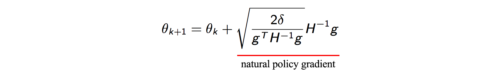
This is what is called a Natural Policy Gradient. We could stop here and use this update rule in our algorithm. But calculating the inverse of the Hessian matrix $H$ that we get is very expensive, especially for large deep networks. Also, the inverse is numerically unstable. So we need to again find some method for approximating it.

Thanks to the Conjugate Gradient (CG) algorithm for this!!

So instead of computing the inverse of $H$, we can solve the below equation -

This can be converted to a quadratic optimization problem and could be solved using the CG algorithm. We transform it into quadratic form by following -

Which is solving for the following equation -

I would not go into the details for the CG algorithm but would like to give intuition behind it.

The CG algorithm is similar to Gradient Ascent but optimizes the problem in fewer iterations. If the model has $P$ parameters, then the CG method solves the problem in at most $P$ iterations. It does this by finding a search direction (in the parameter space) that is orthogonal to all the previous directions. So by doing this, it is not undoing any progress that it made previously (which Gradient Ascent normally does).

Solving this CG problem is much lower in complexity as compared to computing the inverse of $H$. After at most $P$ iterations, we will have the value of $x$ calculated which could be plugged in the update equation for optimization. This gives us a reasonable approximation.

So now we have almost all the pieces of the puzzle and we just need to put them together in one algorithm to form TRPO. But what are we waiting for?

As you would have noticed, we have made a lot of approximations in order to make things feasible. First, we approximated the optimization problem using Taylor polynomial and then approximated the solution for $x$ as a quadratic optimization problem, thereby using CG algorithm to avoid calculating the inverse. These approximations may reintroduce the problem with policy updates and degrade the training. So we need some way to verify that the update we make actually improves performance, and if it does not, we need to find some way to make it do so.

What we use here is something called Line Search in the optimization literature.

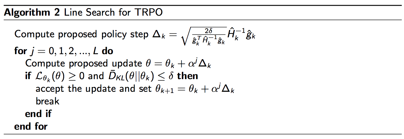
We verify the new policy $\theta_{k+1}$ first by doing a Line Search and then only make the update. We need to verify two things -

1. KL divergence between the policies is less than $\delta$ (maximum allowed value according to the trust region).

2. The surrogate advantage $L$ is greater than or equal to $0$ (Since $L$ is close to the difference between the reward function for two policies for small policy changes).

We introduce a decay factor - $\alpha$ (0 < $\alpha$ < 1). If the current step does not satisfy the two conditions, we decay it by a factor of $\alpha$ and then again check for the two conditions. We continue this until it satisfies the conditions and then use that step to make an update to the policy parameter $\theta$.

By doing so, we take the largest possible step to change the policy parameter $\theta$ such that it does not hurt the performance. This ensures that we find the most optimal point in our trust-region and then continue from there.

So now we have the whole algorithm ready. Following is the Pseudo-code for TRPO -

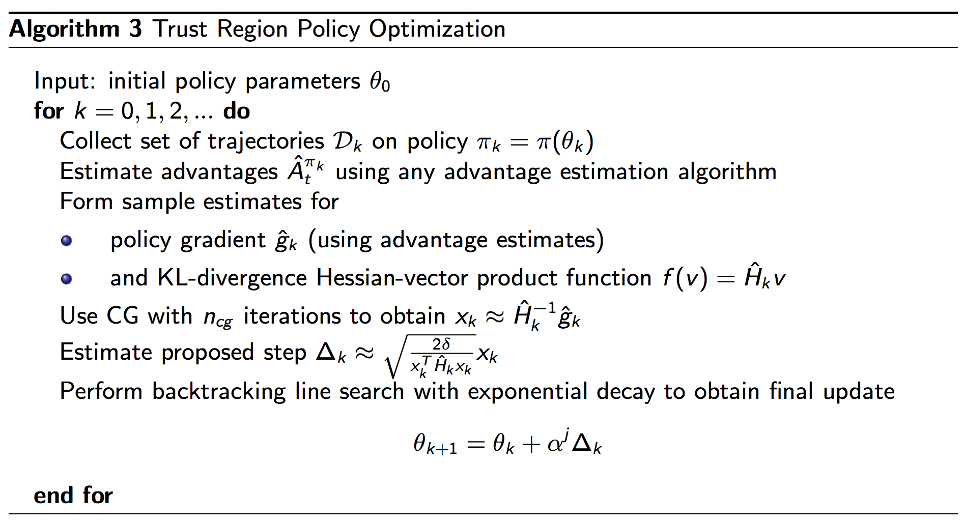
Few points to remember -

Although TRPO offers a lot of theoretical guarantees but does not perform very well on certain RL problems. It performs good for continuous control problems (see TRPO + GAE), while degrading performance on Atari games (which have pixel-based state-inputs) as compared to the benchmark Value-based algorithms. It is still inefficient in terms of computational expenses and sample efficiency, as compared to algorithms like PPO and Actor-Critic based Kronecker-Factored Trust Region (ACKTR).

In terms of computational cost, the conjugate gradient algorithm allows us to approximate the Hessian inverse without actually computing it, but we still need to find the Hessian matrix. This is again quite expensive and is generally avoided by using the Fisher Information Matrix (FIM) as an approximation to the second-derivative of the KL-divergence. Hence we have the following optimization problem -

Despite of these downsides, TRPO gives us a new and possibly better way to look at the Policy Gradients and scope for a lot of improvement in the future.

Finally, we arrive at the end after going through so many theoretical methods in optimization and probability theory. Hope you enjoyed it :)