Survey on Adversarial Attacks and Defenses in Reinforcement Learning
Survey on Adversarial attacks and defenses in Reinforcement Learning
This post contains various adversarial attacks and defensive strategies in Machine Learning, with a specific focus on Reinforcement Learning.
- Introduction
- Pixel-based attacks
- Attacking by training Adversarial policies
- Defenses against Adversarial attacks
- End Thoughts
- References and Further reading
Introduction
To a large extent, robustness in Reinforcement Learning (RL) depends upon the robustness of the function approximator network, which is used to output the Value functions or the action probabilities. The most common class of function approximators that are used in RL are Neural Networks (NN). Hence, the research works which aim to exploit the vulnerabilities of the Neural Nets and explore the potential defenses for them in the supervised learning setting are also applicable in RL.
Apart from that, there are few other attacks which do not rely on the function approximator, and are caused due to the complications that arise during training and optimization in Multi-Agent Reinforcement Learning (MARL). Such methods are specifically applicable in RL settings. We’ll see attacks in both settings.
Broadly there are two types of attacks -
Pixel-based attacks
These types of attacks change the input observation of the function approximator (Neural Net in our case). If the input to the neural network is in the form of pixels, the adversary can make carefully calculated perturbations to the pixels, so that the RL agent picks an incorrect action, which might lead the agent to a bad state. The perturbation is made such that the change in the input image is imperceptible to the human eye. This type of attack was initially introduced in Computer Vision settings and later extended to RL.
The main hypothesis behind such attacks is our Machine Learning (ML) models being too linear or piecewise linear functions of the input (more on this later). Though this phenomenon was initially observed in Neural Nets, it is not a characteristic of Deep Learning. It is fundamental to our simplest ML models. And because Neural Nets are essentially made up of all these linear models (linearly combining and using an activation function like ReLU), they inherit these flaws.
This attack is also applicable in RL settings as again the Neural Nets or other traditional ML models are used to approximate the value functions and the policies. Hence the models are again fooled.
Attacking by training an Adversarial policy
This type of attack has been introduced recently. The attacker trains an adversarial policy for the opponent, which took certain actions that generated natural observations that were adversarial to the victim policy. Don’t worry if you don’t understand it now :P. We’ll discuss this in detail in the later sections.
We will see both the categories one by one -
Pixel-based attacks
These types of attacks focus on attacking the vulnerabilities in the function approximator. But first of all, let us see what does robustness of a Neural Network or any other model in general mean - Robustness of a model is defined as a measure of how easy it is to find adversarial examples that are close to their original inputs.
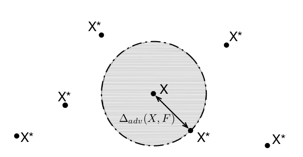
In the above figure, $X$ is the original input sample and $F$ is the network. The expected value (with respect to the input distribution) of the radius of the circle is defined as the robustness of the network.
\[\rho_{adv} (F) = \mathbb{E}_\mu[\Delta_{adv}(X, F)]\]Here $\rho$ means robustness, and $\mu$ is the input distribution. It is important to note that the class of the input example $X$ remains same inside the circle. The points outside correspond to the adversarial examples created by modifying the pixel-values of $X$.
Remember that the attacks that generate adversarial examples should apply minimum distortion to the original inputs, and still be able to fool the model, otherwise the examples would be distinguishable by humans.
Most of these attacks are studied in Computer Vision but can be applied in a similar fashion in RL, where the input state-space to the Neural Net is the pixels. The papers follow different approaches but a common goal. The goal is to -
-
Find the input features that are most sensitive to class change (change in the action executed by the agent in RL).
-
Make a perturbation, i.e, change the pixels slightly such that the network misclassifies the input but the change is visually imperceptible to humans. For RL, it would be equivalent to forcing the agent to take wrong action.
In short, they focus on making small $L_p$ norm perturbations to the image. Also, all the attacks that we discuss do not tamper with the training process in any way. Data-poisoning attacks that tamper do so are also very popular, especially in Online and Lifelong learning settings, where the agent continuously keeps learning, and there is no clear distinction between training and testing. However, in this article, we consider only the attacks made after the system is ready to be deployed, and its parameters are frozen. Essentially, all these attacks are made during the test time.
INTRIGUING PROPERTIES OF NEURAL NETWORKS (Szegedy et al. 2014a)
This is probably the first paper discovering such attacks in the context of Neural Nets. The authors generate adversarial examples using box-constrained L-BFGS. They provide results on MNIST and ImageNet datasets. They argue that adversarial examples represent low probability pockets in the manifold represented by the network, which are hard to efficiently find by simply randomly sampling the input around a given an example. They also found that the same adversarial example would be misclassified by different models trained with different hyperparameter settings, or trained on disjoint training sets. They refer to it as the transferability property of adversarial examples.
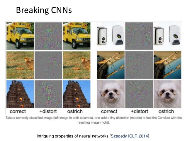
However, the authors do not provide a concrete explanation of the reason behind such adversarial examples occur. If the model is able to generalize well, how can it get confused with the inputs that look almost similar to the clean examples?. They say that the adversarial examples in the input space are like rational numbers in the real number space – sparse yet dense. They argue that an adversarial example has very less probability (hence rarely occurs in the test set), and yet dense because we can find an adversarial example corresponding to almost every clean example in the test set.
EXPLAINING AND HARNESSING ADVERSARIAL EXAMPLES (Goodfellow et al. 2015)
This paper proposes a novel way of creating adversarial examples very fast. They propose Fast Gradient Sign Method (FGSM) harness adversarial samples. This method works by taking the sign of the gradient of the loss function with respect to the input. They use the max norm constraint in which each input pixel is changed by an amount of no more than $\epsilon$. This perturbation is then added to or subtracted from each pixel (depending upon the sign of the gradient). This process can be repeated until the distortion becomes human-recognizable, or the network misclassifies the image.
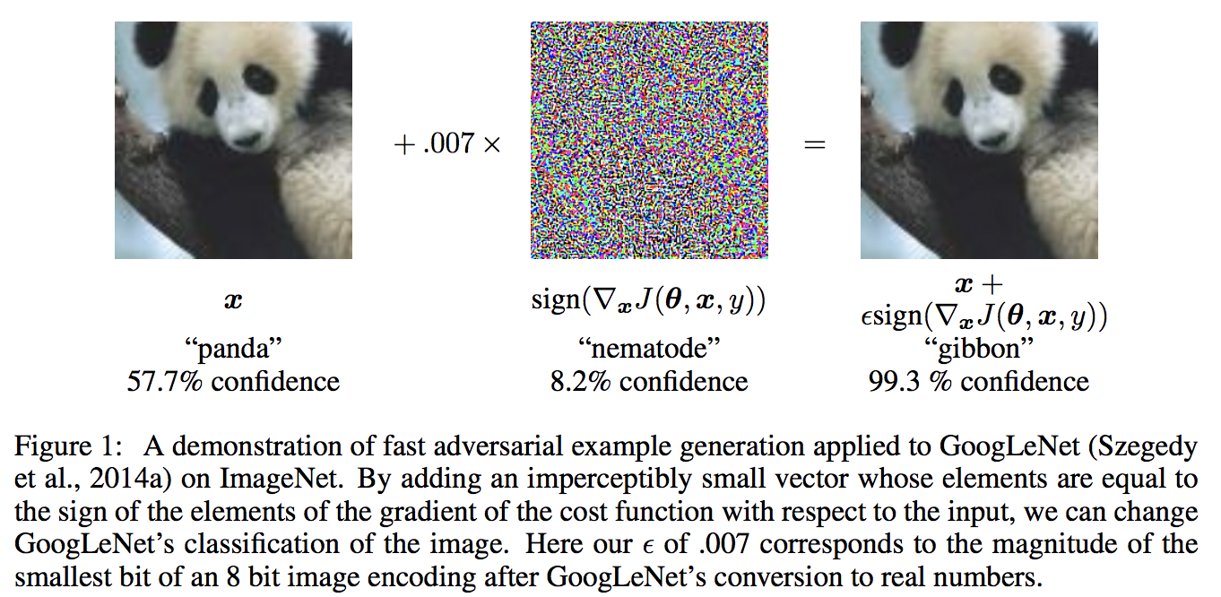
FGSM works as a result of the hypothesis the authors propose for the occurrence of adversarial examples. Earlier, it was thought that adversarial examples are a result of overfitting and the model being highly non-linear. However, empirical results showed something else. If the above notion of overfitting was true, then we should get different random adversarial example points in the input space if we retrain the model with different hyperparameters or train a slightly different architecture model. But it was found that the same example would be misclassified by many models and they would assign the same class to it.
Following is a paragraph from the paper.
”””
Why should multiple extremely non-linear models with excess capacity consistently label out-of-distribution points in the same way? This behavior is especially surprising from the view of the hypothesis that adversarial examples finely tile space like the rational numbers among the reals, because in this view adversarial examples are common but occur only at very precise locations.
Under the linear view, adversarial examples occur in broad subspaces. The direction η need only have a positive dot product with the gradient of the cost function, and need only be large enough.
”””
So the authors proposed a new hypothesis for the cause of adversarial examples to be these models being highly linear or piecewise linear functions of the inputs, and extrapolating in a linear fashion, thus exhibiting high confidence at the points it has not seen in the training set. The adversarial examples exist in broad subspaces of the input space. The adversary need not know the exact location of the point in the space but just needs to find a direction (gradient of the cost function) giving a large positive dot product with the perturbation. In fact, if we take the difference between an adversarial example and a clean example, we have a direction in the input space, and adding that to a clean example would almost always result in an adversarial example.
In summary, this paper gives a novel method of generating adversarial examples very fast and gives a possible explanation for the existence and generalizability of adversarial examples.
Another explanation for FGSM in simple words is -
In Machine Learning, we use the gradient of the cost function with respect to the model parameters to optimize them to minimize the cost keeping the input to the model fixed, whereas,
For generating adversarial examples, we do the opposite. We try to maximize the cost by moving the input values in the direction of the gradient of the cost function with respect to the input, keeping the parameters of the model fixed.
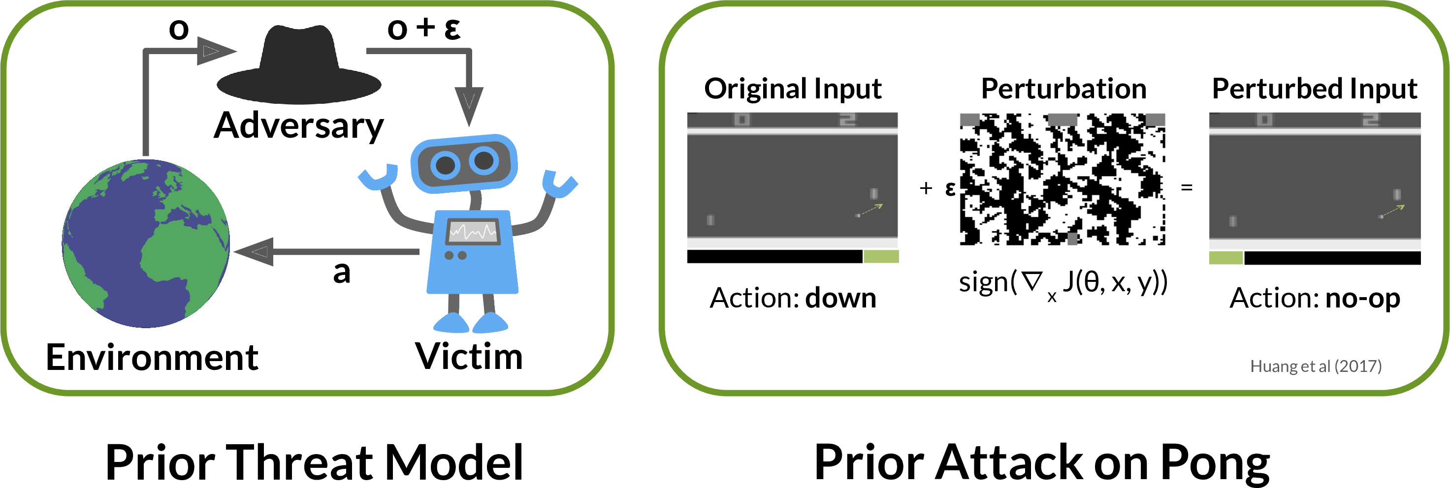
ADVERSARIAL ATTACKS ON NEURAL NETWORK POLICIES (Huang et al. 2017)
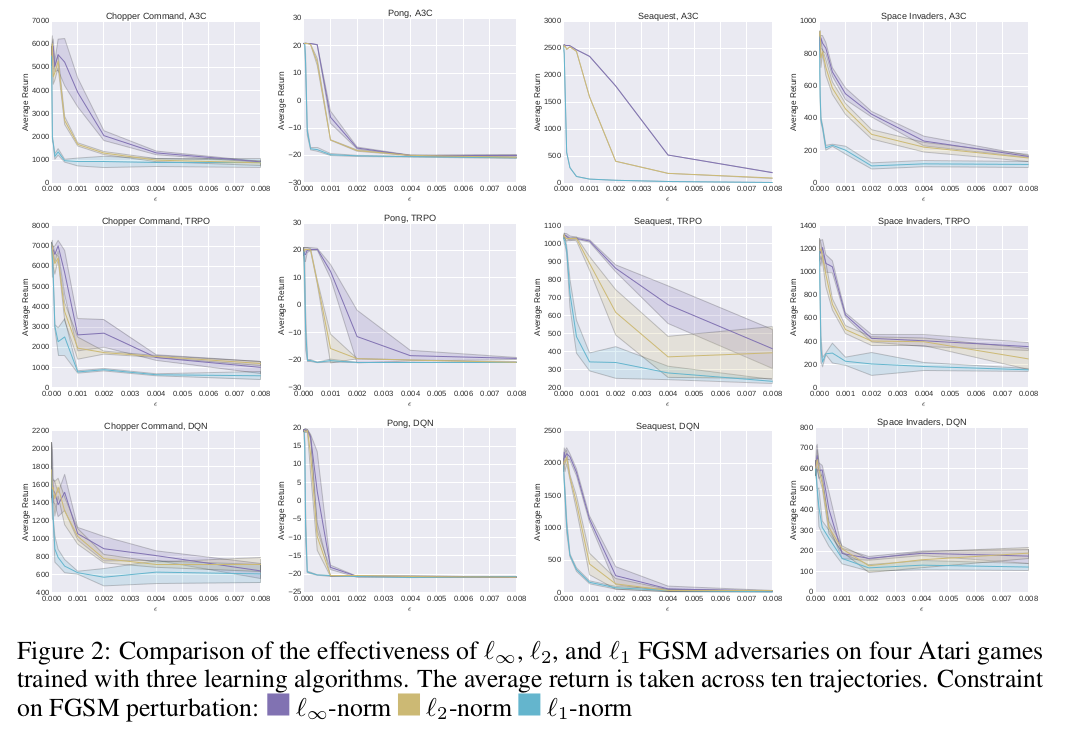
This is the first paper showing the existence of adversarial attacks in Reinforcement Learning. Here they show attacks on three RL algorithms - DQN, TRPO, and A3C in Atari environments in both White-box (i.e., the adversary has access to the training environment, Neural Net architecture, parameters, hyperparameters, and the training algorithm) and Black-box settings. The approach followed is the same as FGSM (as the state input to the Neural Net function approximator are the raw pixels), and they do it with different $L_p$ norms. Here the loss is computed as the cross-entropy loss function between the output action probabilities and the action with the highest action probability, in case of policy-based methods. For DQN, the output Q-values are converted to a probability distribution using the softmax function with temperature. These attacks are able to decrease the rewards per episode by a considerable amount by making the RL agent take the wrong action in various situations.
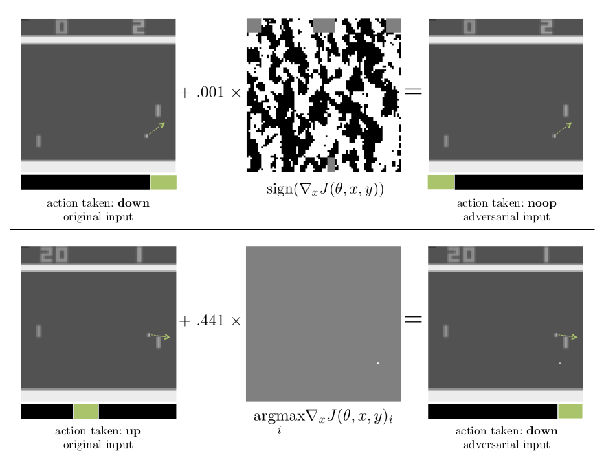
The attack is similar to the gradient attack in Computer Vision (as discussed above). There the objective was to make the network misclassify the image, while here the same thing holds with actions. The authors provide the results for white-box as well as black-box settings. The latter is divided into two parts -
-
Transferability across policies - Adversary has all the knowledge as in the case of white-box attacks except the random initialization of the target policy network.
-
Transferability across algorithms - Adversary has no knowledge of the training algorithm or hyperparameters.
Some important conclusions from this paper -
-
The attack methods like FGSM (and ones further we will discuss) are applicable in RL domains also. This is because the root cause of these attacks is not related to any specific field; instead, they apply to all the models in Machine Learning, which are linear or literally piecewise linear functions of the inputs. Neural Networks come under this category, hence are vulnerable to them. Since RL can only be applied in real-world problems with continuous state and action spaces using these function approximators, these attacks can also confuse well-trained RL agents that take state input in the form of pixels.
-
DQN tends to be more vulnerable to adversarial attacks as compared to policy gradient methods like TRPO and A3C.
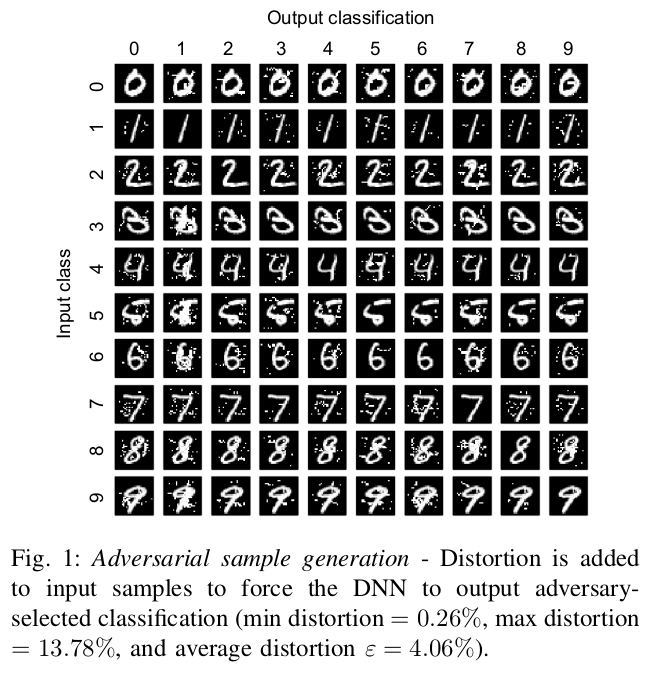
THE LIMITATIONS OF DEEP LEARNING IN ADVERSARIAL SETTINGS (Papernot et al. 2016)
This paper proposes a slightly different approach to craft adversarial samples. Unlike Goodfellow et al. 2015, this method does not alter all the pixels by equal amounts. The adversaries craft the examples by carefully finding the input dimensions, changing, which will have the most impact on class change. Hence this attack fools the network in the minimum required perturbation only to the pixels that can cause class change with higher probability.
Here, instead of computing the gradient of the loss by backpropagation, the adversary finds the gradient of the Neural Net output with respect to the input as a forward derivative, i.e., the Jacobian matrix of the function learned by the Neural Net by recursively computing the gradient for each layer in a forward run. The authors do this as this enables finding input components that lead to significant changes in the network outputs. This is followed by constructing adversarial saliency maps, which act as heuristics to estimate the pixels to perturb.
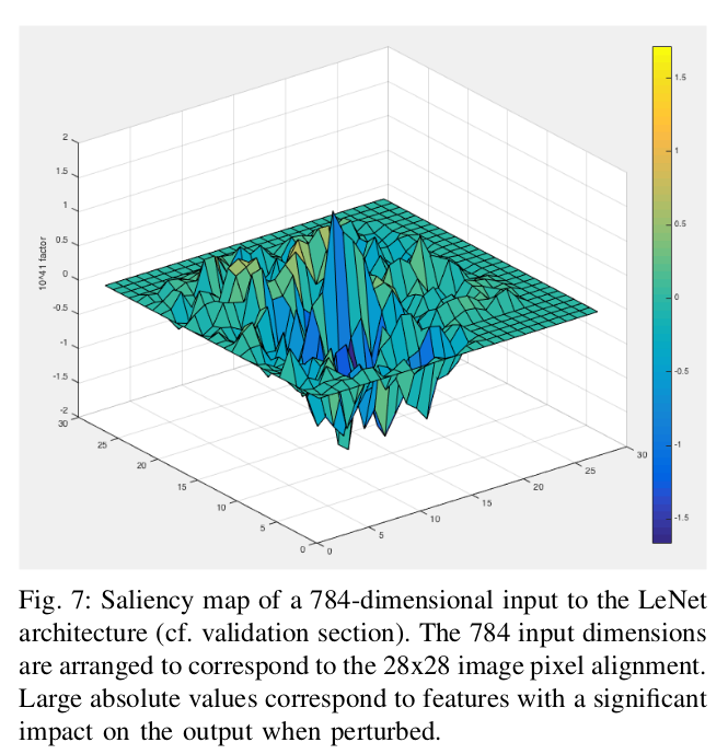
One important thing to note in this approach is that unlike Goodfellow et al. 2015, it implicitly enables source-target misclassification, i.e., forcing the output classification of a specified input to be a specific target class.
The reason for this being that here we compute the Jacobian of the function which the network is trying to learn. This derivative (Jacobian) basically tells how much an output neuron changes if we change an input pixel, which gives us a direction in which we can increase or decrease the probability of any output class. Hence we can increase or decrease an input pixel in such a way that it increases the probability of a certain target class and decreases the probabilities of others. This gives a stronger advantage to the adversary in not only making the Neural Net misclassify the input but also leading it to a target class.
This form of attack can have a significant impact when applied to RL settings. This is due to the inherent closed loop nature of an RL problem. An agent’s actions at the current time step determine what next state will it be in and then again the actions in the next state and so on, this loop continues, making RL a sequential problem. There can be certain scenarios where the attacker forces the agent to take a wrong action in some critical state, doing which would lead to a bad policy. Now say considering Policy Gradient approaches, new data (trajectories) would be collected using this bad policy, and it would finally lead to a collapse in the performance.
TACTICS OF ADVERSARIAL ATTACK ON DEEP REINFORCEMENT LEARNING AGENTS (Lin et al. 2017)
Here the authors argue that the previous work for adversarial attacks in Deep RL (Huang et al. 2017) ignores certain important factors. The attack needs to be minimal in both spatial as well as temporal domains, and previous work says nothing about minimizing the number of timesteps in which attack is made. Hence they give two novel tactics for attacking Deep RL.
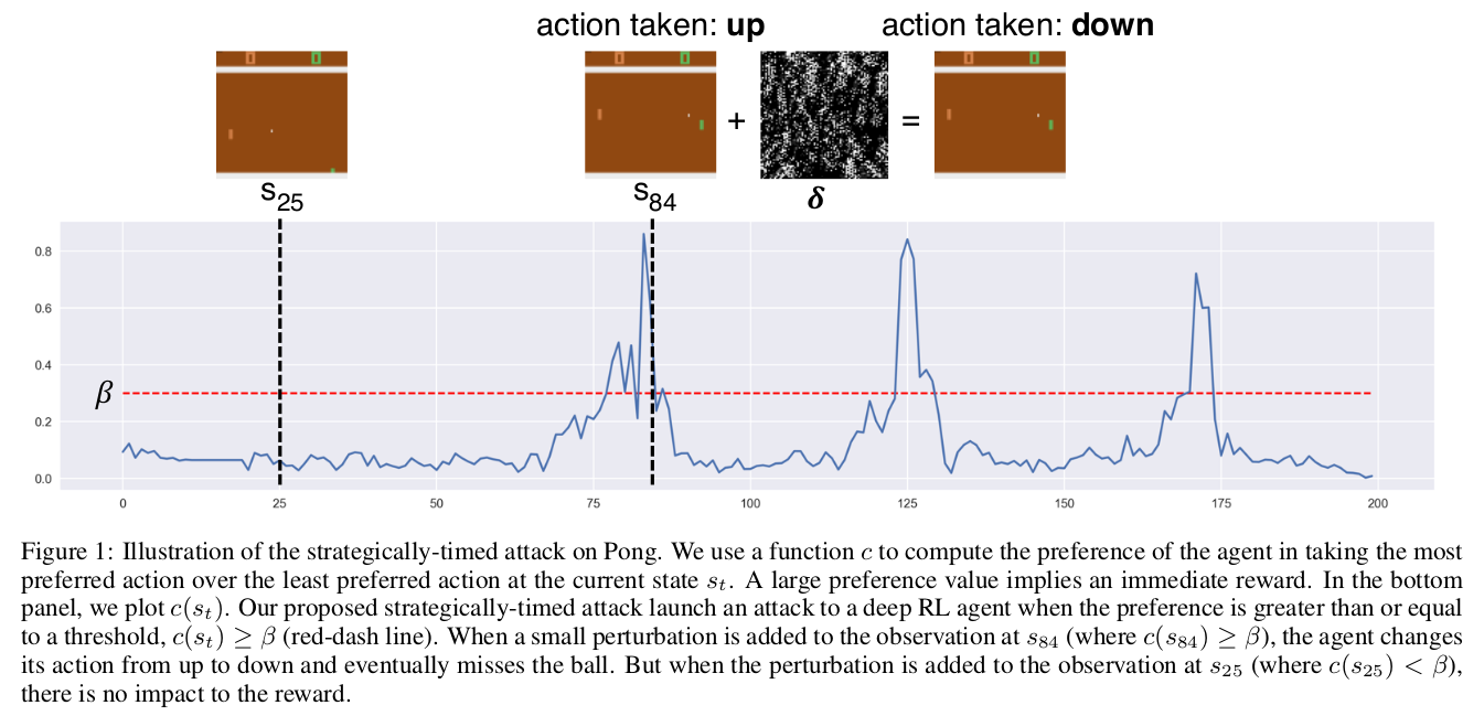
Strategically-timed attack
This attack accounts for the minimal total temporal perturbation of the input state. It is based on a simple observation: The adversary should attack the RL agent only in critical situations where the agent has a very high probability of taking a particular action. A simple analogy can be given in the case of Pong. At the time instants when the ball is away from the agent and moving towards the opponent, intuitively, the probability of the agent taking any action should be more or less uniform. Making a perturbation at these timesteps does not make sense.
Instead, the time steps when the ball is very near to the agent padel, its probability of taking a certain action is very high. This is because a well-trained policy would take the correct action most of the time. Hence attacking at this time instant is likely to provoke the agent to take another action, thereby missing the ball and getting a negative reward.
The authors make this attack by framing a mixed integer programming problem, which is difficult to solve. So instead, they use a Heuristic to measure the time steps in which to attack. They measure the difference between the action probabilities of the most preferred and the least preferred action. If it is more than a certain threshold $\beta$, they attack (add perturbation), otherwise not. For DQN, this is calculated by passing Q-values through the softmax function with temperature. Once the difference is more than the threshold, the adversary uses the Carlini-Wagner method to attack, where the target class is the least preferred action before adding the perturbation.
For limiting the total number of attacks, there is an upper bound to the total number of time steps in which the adversary can attack. Results show that it is possible to reach the same attack success rate as in Huang et al. 2017 while attacking only 25% of the total time steps per episode on average.
Enchanting attack
This attack is based on the closed loop and sequential property in RL, where the current action affects the next state and so on. It lures the agent to a particular state of the adversary’s choice. This is accomplished by using a planning algorithm (to plan the sequence of actions that would ultimately lead the agent to the target state) and a Deep Generative model (for simulation and predicting the model). In the paper, the authors assume that the adversary can take full control of the agent and make it take any action at any time step.
The first step is to force the agent to take the first planned action in the current state. This is achieved by the Carlini-Wagner attack to craft the perturbed state leading the agent to a new state from where this process is repeated until it reaches the target state.
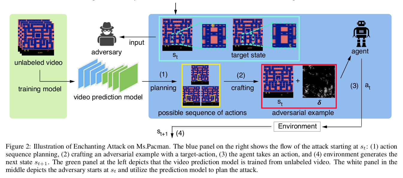
This type of attack can be extremely beneficial for the adversary in some cases like autonomous driving where it can lead the car (agent) to a bad state like hitting an obstacle and causing an accident. It also seems to be a much more promising and strategic attack than others to allow the adversary to exploit the agent to its fullest potential.
Note: There is one more type of Pixel-based attack which is stronger than all of the
approaches discussed above. We'll discuss that after Defensive Distillation in the
Adversarial defenses section.
Attacking by training an Adversarial Policy
All the forms of attacks discussed above hurt the performance of the RL agent by making adversarial perturbations to the image observations. However, real-world RL agents inhabit natural environments populated by other agents, including humans, who can modify another agent’s observations via their actions. In such cases, Pixel-based attacks won’t be much useful. To give a concrete example, say we have a mixed cooperative-competitive environment with N agents, where the agents are distributed in teams. Here the agents in a team should cooperate with each other to win and simultaneously compete with the agents in the other teams. These scenarios are common when we think about large-scale applications of Deep RL like OpenAI Five’s Dota playing agents, etc. In such environments, attacking by training an adversarial policy could make the performance worse.
As a result, it would be interesting to explore the consequences of adversarial observations on RL agents, especially the ones deployed in the simulated/real world. Again, here we will discuss only the attacks at the test time.
ADVERSARIAL POLICIES: ATTACKING DEEP REINFORCEMENT LEARNING (Gleave et al. 2020)
Note: Related Work section of this paper contains many other existing approaches
This paper follows a different approach towards attacking well-trained RL agents from what we have seen till now. Unlike an indirect approach of attacking Deep RL by exploiting the vulnerabilities in the Deep Neural Nets, this paper trains an adversarial policy in multi-agent competitive zero-sum environments directly to confuse/fool the agent (also referred to as the victim), thereby decreasing the positive reward gained. The paper is able to successfully attack the state-of-the-art (SOTA) agents trained via self-play to be robust to opponents, especially in high-dimensional continuous control environments, despite the adversarial policy trained for less than 3% of the time steps than the victim and generating seemingly random behavior.
Let us look at a detailed analysis of the paper -
Previous works on adversarial attacks in Deep RL have used the same image perturbation approach, which was initially proposed in the context of Computer Vision. However, as discussed before, the real-world deployments of RL agents are in natural environments populated by other agents, including humans. So a more realistic attack would be to train an adversarial policy that can take actions that generate natural observations that are adversarial to the victim.
A motivation for this attack from the paper is -
”””
RL has been applied in settings as varied as autonomous driving (Dosovitskiy et al., 2017), negotiation (Lewis et al., 2017) and automated trading (Noonan, 2017). In domains such as these, the attacker cannot usually directly modify the victim policy’s input. For example, in autonomous driving pedestrians and other drivers can take actions in the world that affect the camera image, but only in a physically realistic fashion. They cannot add noise to arbitrary pixels, or make a building disappear. Similarly, in financial trading an attacker can send orders to an exchange which will appear in the victim’s market data feed, but the attacker cannot modify observations of a third party’s orders.
”””
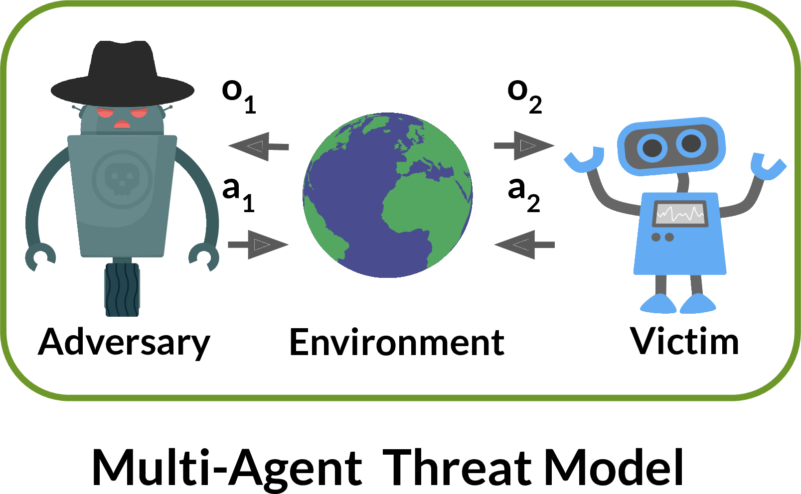
The method in this paper seems to be more appropriate for attacking Deep RL in actual deployment domains. A key point here is that the adversary trains its policy in a black-box scenario where it can just give observation input to the victim (by its actions) and receive the output from it. The key difference in this approach is using a physically realistic threat model that disallows direct modifications of the victim’s observations.
Setup
The victim is modeled as playing against an opponent in a two-player Markov game. The opponent is called an adversary when it can control the victim. The authors frame a two-player Partially Observed Markov Decision Process (POMDP) for this. The environment is partially observed as in most Multi-Agent RL settings. The adversary is allowed unlimited black-box access to the actions sampled from the victim policy, which is kept as fixed while making an attack. Hence the problem reduces to a single-agent game as the victim policy is fixed.
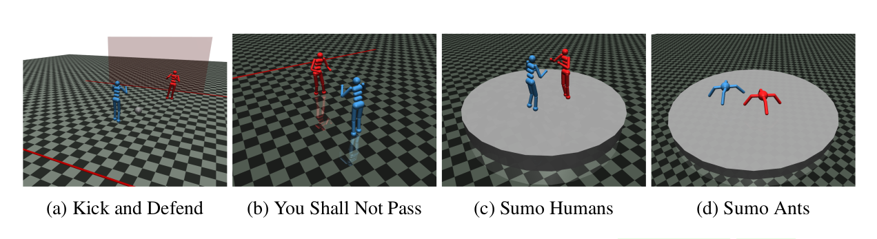
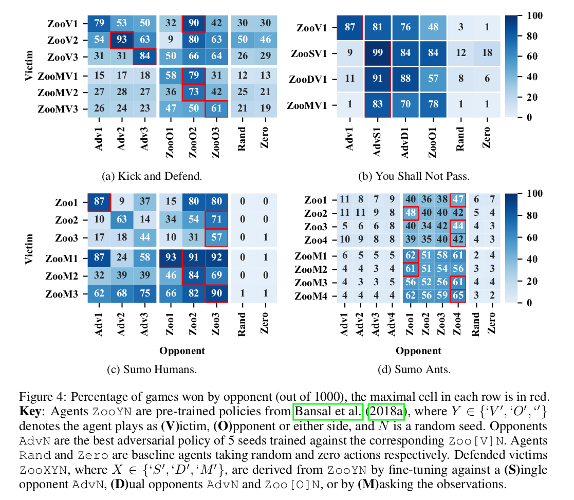
The experiments are carried out in zero-sum environments using the MuJoCo robotics simulator, as introduced in Bansal et al. (2018a). The environments and the rules for the game are described in the paper. The victim policies are also taken from the pre-trained parameters in Bansal et al. (2018a), which are trained to be robust to opponents via self-play. The environments used in the paper are - Kick and Defend, You shall not pass, Sumo Humans, and Sumo Ants.
Training the adversarial policy
Although Bansal et al. (2018a) have pre-trained opponents as well, which try to fail the victim from doing their tasks in the respective environments, the authors trained a new adversarial policy. They did this using the PPO algorithm, giving the adversary sparse positive reward when it wins against the victim and negative if it loses or ties. They train it for 20 million time steps, which is less than 3% of the time steps the victims were trained.
Results and Observations
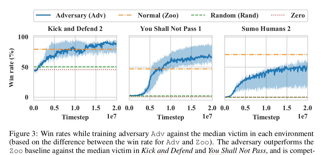
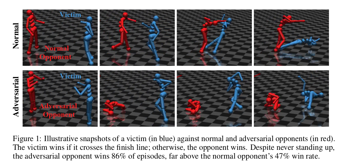
The adversarial policy succeeds in most environments and performs better than Rand, Zero, and Zoo* opponents. Here an important observation is that the adversarial policy wins against the victims not by becoming strong opponents (i.e., performing the intended actions like blocking the goal) in general but instead taking actions that generated natural observations that were adversarial to the victim policy. For instance, in Kick and Defend and You shall not pass, the adversary never stands up and learns to lie down in contorted positions on the ground. This confuses the victim and forces it to take wrong actions. In Sumo Humans, if the adversary does the same, it loses the game, so it learns an even interesting strategy to kneel down in the center of the sumo ring in a stable position. In the former two environments, the adversary’s win rate surpasses all the other types of opponents, and in Sumo Humans, it is competitive and performs close to the Zoo opponents.
The victim does not fail just because the observations generated by the adversary are off its training distribution. This is confirmed by using two off-distribution opponent policies - Rand (takes random actions) and Zero (lifeless policy exerting zero control). The victim is fairly robust to such off-distribution policies until they are specifically adversarially optimized.
Masked Policies
This is an interesting methodology adopted in the paper to empirically show that the adversaries win by natural observations that are adversarial to the victim, and activations are very different from the ones generated by normal opponents.
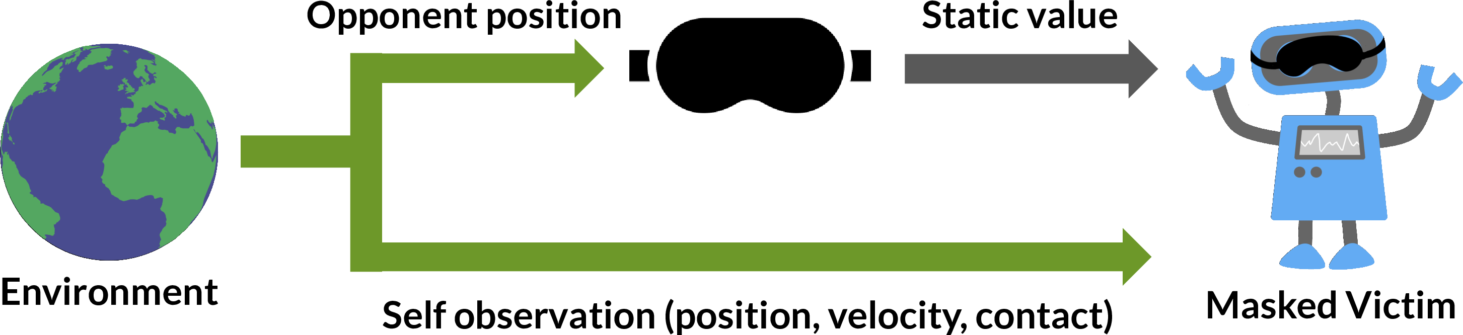
The authors compare the performance of the masked and the normal victims against the adversarial and the normal opponents. Masked victim means that the observation input of the victim is set to some static initial opponent position. One would normally expect the victim to perform badly when the position of the opponent and the actions it takes are “invisible”. This is indeed the case with the normal opponent. The masked victim performs poorly against it. However, the performance of the masked victim against the adversary is seen to improve as compared to the unmasked victim.
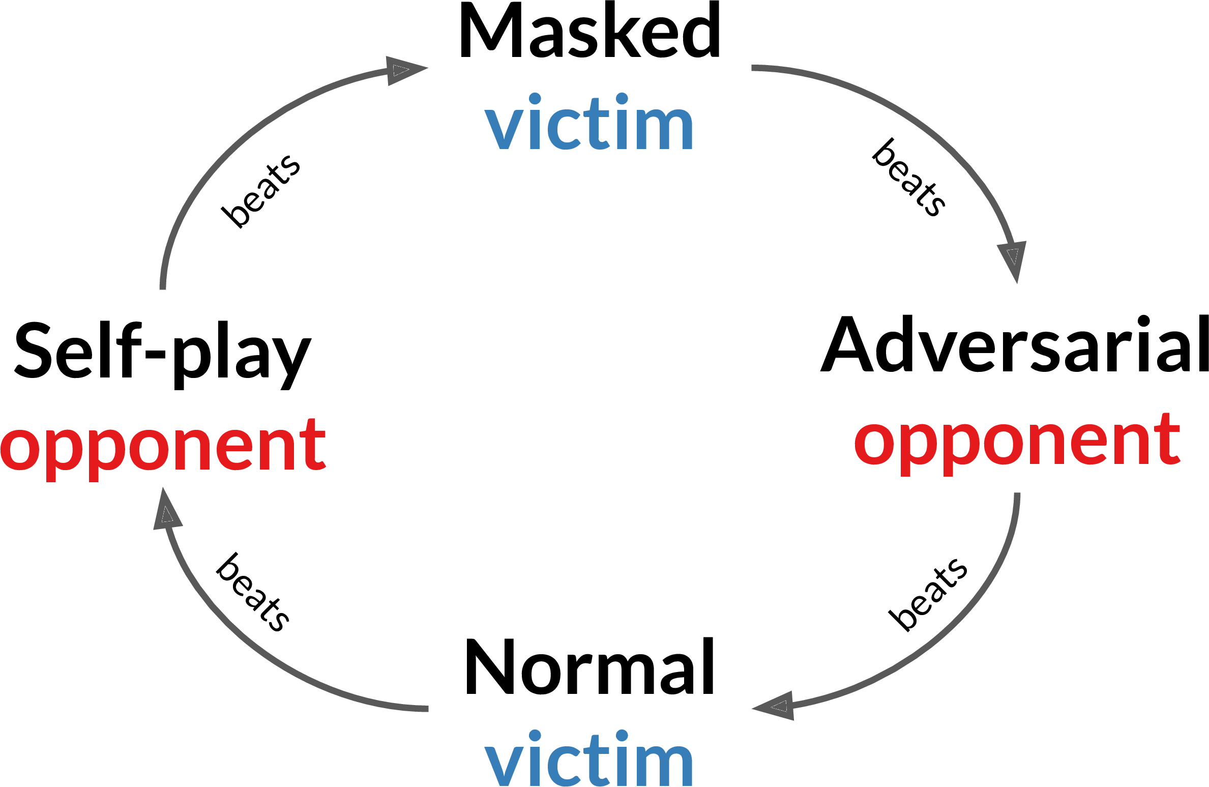
This also leads us to an important observation. All these games discussed above are transitive in nature, i.e., a high-ranked professional player should intuitively outperform a low-ranked amateur player. However, here the adversary wins not by physically interfering with the victim or becoming strong opponents, but instead placing it into positions of which the victim is not able to make sense. This suggests highly non-transitive relationships between adversarial policies, victims, and masked victims. This is similar to an out-of-syllabus question that is specifically designed to confuse the student.
Effects of Dimensionality
In Pixel-based attacks, it has been observed that classifiers with high-dimensional inputs are more vulnerable to adversarial examples. A similar thing is observed here. The authors compare the performance of the adversary in two types of environments in the Sumo game. One with Sumo Humanoid and the other as Sumo Ant quadrupedal robots. In the former case, the adversary has access to $P$ = 24 dimensions of the total observation space that it can influence, while the latter has only $P$ = 15. $P$ is the adversarial agent’s joint position. As we can see in the matrix tables illustrated in the figures, the damage caused by the adversary in the first case is more than in the second.
Why are victim observations adversarial?
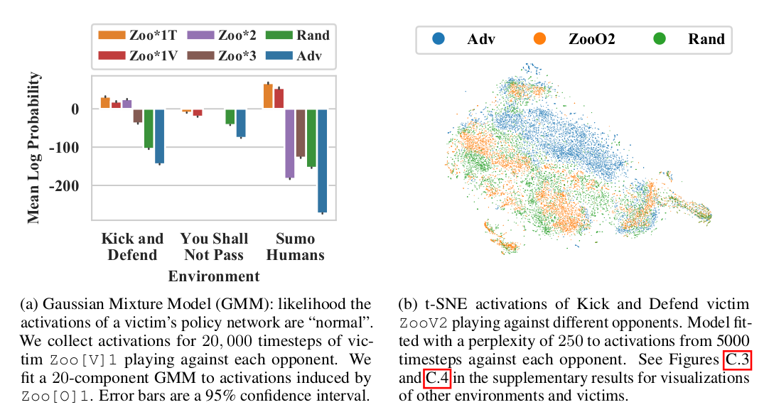
From the Mask-policy experiment, we know that adversarial policies win by creating natural observations that are adversarial to the victim. But why are the victim observations adversarial? For this, the authors plot the activations of the victim policy using Gaussian Mixture Model (GMM) and t-SNE visualization. They observe that the activations induced by adversarial policy substantially differ from the ones induced by normal opponents.
The GMM shows the likelihood of the victim’s policy network activations being “normal”. We observe highly negative mean log probabilities for the victim against an adversarial policy. Also in the t-SNE plots, the activations against an adversarial policy are more dispersed as compared to the random policy Rand, which more widely spread than ZooO2
Why are these attacks possible and Why should we care?
Although the empirical results are quite strong, the appropriate reason behind these attacks and the seeming vulnerabilities of the agent policies might not be clear. What is the factor responsible for this observed behavior – Is it the algorithm that is used to train the agents or the way in which the problem is formulated (Markov games) or is it the optimization procedure?
To answer this question, let us dive a bit deeper into another question :P - What does it mean for the agent policies to “converge” in competitive multi-agent environments?
So the notion of convergence in single-agent RL is clear. It can either be in terms of policies that gain maximal reward out of finite set of all possible policies or a policy that achieves certain desirable target/goal/behavior. As we can see, the objective is clear in such cases. So there is no doubt about convergent behavior. However, in the case of Multi-agent RL, considering competitive scenarios, the notion of the final objective is not clear. It depends on the situation and application.
However, most of the time, the goal is to achieve a Nash Equilibria. It is defined as follows -
\[\begin{align}&\text{If there are N agents in Nash equilibria, it means that none of the agents has any} \\ \\ &\text{incentive to unilaterally change its strategy/policy with the strategies/policies of } \\ \\ &\text{all other N - 1 agents remaining the same}\end{align}\]There can be multiple possible Nash equilibria in a game. But what does this got to do with the attacks?
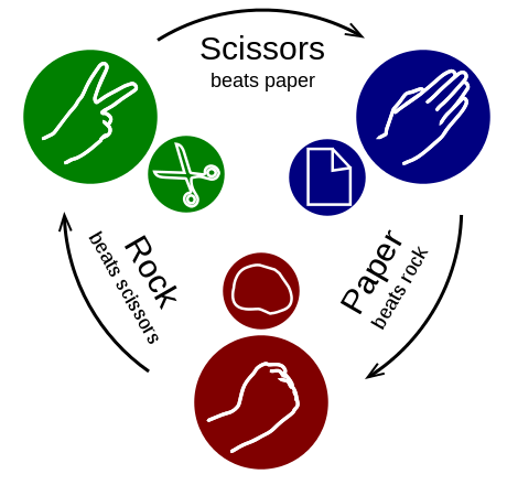
Remember the cyclic non-transitive relationship that we observed among the adversarial, normal opponent, masked, and victim policies? This behavior is similar to what we see in Rock-Paper-Scissors (RPS). There does not exist a pure-startegy Nash in RPS. Say there is a situation where player 1 has rock, and player 2 has paper. Following this, the player 2 wins, so it would not change its strategy. For player 1, switching its move to scissors, provided the player 2 stays with paper, will be more rewarding, and hence the two players are not in Nash. We will have a cyclic behavior like - paper, scissors, rock, paper, scissors, rock…... The same is true in case of the policies we have seen.
In more formal words, if Agent1’s parameter vector is $x\epsilon\mathbb{R}^m$ and Agent2’s $y\epsilon\mathbb{R}^n$, then we need to find a set of the parameters in the $\mathbb{R}^{mxn}$ space such that the two agents play a Nash. If the victim policy plays a Nash equilibrium, it would not be exploitable by any adversary. Self-play is one popular method for achieving this condition, and it has produced highly capable AI systems like AlphaGo and OpenAI Five. However, it is also well known that self-play may not always converge to Nash, as it happened in this case.
This suggests that we might need to look again at the optimization procedure used to train the policies. Better competitive optimization would help in closing Nash fast and more efficiently. However, the authors mention that they expect this attack procedure to succeed even if the policies converge to a local Nash as the adversary is trained starting from a random point that is likely outside the victim’s attractive basin.
Now, why should we care about these attacks? The then SOTA self-play policies given by Bansal et al. (2018a) exhibit highly complex emergent behavior and even transferability of the policies across environments. Isn’t it enough? The answer is NO!
Indeed the policies proposed by Bansal et al. (2018a) have extremely good average-case performance. However, their worst-case performance is terrible. Considering adversaries in any training procedure is very important if the system is to be deployed for testing in real-world domains. Hence it is important that we design policies that not only perform well in usual normal conditions but also that can adapt to changing opponent behaviors and/or adversarial changes in the environment.
Defenses against Adversarial policies
The authors tried basic Adversarial training as a defense to these policies, i.e, training the victim explicitly against the adversary. The authors use two types of adversarial training - single and dual. The victim is just trained against the adversary in the former, while against both an adversarial and normal zoo policy randomly picked at the beginning of each episode. However, they found that even if the victim becomes robust to that adversary, it is not robust to the attack method. They are able to find another adversarial policy that fails the victim, which even transfers to the previous victim (i.e., before adversarial training). However, the nature of the new adversarial policy is very different from the previous one. The adversarial policy observed previously performs unconventional and non-intuitive moves to fool the victim. But the new policy has to physically interfere by tripping the victim. This suggests the scope of Iterative Adversarial training for resisting these attacks.
Till now, there is no concrete work in defenses in such attacks and is left to future work. Adversarial training seems to be promising but does not generalize well to all kinds of adversaries. The authors also suggest population-based training where the victims are continually trained against new types of opponents to promote diversity, and trained against a single opponent for a prolonged time to avoid local equilibria.
Conclusions and Discussions
In conclusion, this paper makes three key contributions. First, it proposes a novel Multi-agent threat model of natural adversarial observations produced by an adversarial policy taking actions in a shared environment. Second, they demonstrate that adversarial policies exist in a range of zero-sum simulated robotics games against SOTA victims trained via self-play to be robust to adversaries. Third, they verify the adversarial policies win by confusing the victim, and not by learning a generally strong policy. Specifically, they find the adversary induces highly off-distribution activations in the victim, and that victim performance increases when it is blind to the adversary’s position.
Lastly following is a paragraph from the paper which gives a few important points to keep in mind regarding future work -
”””
While it may at first appear unsurprising that a policy trained as an adversary against another RL policy would be able to exploit it, we believe that this observation is highly significant. The policies we have attacked were explicitly trained via self-play to be robust. Although it is known that self-play with deep RL may not converge, or converge only to a local rather than global Nash, self-play has been used with great success in a number of works focused on playing adversarial games directly against humans (Silver et al., 2018; OpenAI, 2018). Our work shows that even apparently strong self-play policies can harbor serious but hard to find failure modes, demonstrating these theoretical limitations are practically relevant and highlighting the need for careful testing.
Overall, we are excited about the implications the adversarial policy model has for the robustness, security, and understanding of deep RL policies. Our results show the existence of a previously unrecognized problem in deep RL, and we hope this work encourages other researchers to investigate this area further.
”””
Now let us see some defense systems against the attacks we have discussed.
Defenses against Adversarial attacks
Many defenses have been proposed to counter these adversarial attacks and make the function approximators (Neural Nets) robust. However, there is no single defense yet which can successfully guarantee protection against all the attacks introduced till now. Here we discuss two such defenses -
Adversarial training
In its most elementary form, this means training the network/policy by generating adversarial examples. This tends to work up to some extent but is not applicable in all situations. Many other efficient and modified forms of Adversarial training have also been introduced. Some of them are -
Ensemble Adversarial training
The models trained via Vanilla Adversarial training can defend weak perturbations but cannot defend against the strong ones. In the Ensemble approach, we train the networks by utilizing several pre-trained vanilla networks to generate one-step adversarial examples. This enhances the training data with perturbations transferred from other static pre-trained models. Doing so makes the networks more robust to Black-Box adversaries, which can train their models and generate adversarial examples that successfully transfer to the actual model. The models trained via this approach have strong black-box robustness to attacks on ImageNet.
We can also extend this procedure to Iterative Ensemble Adversarial training, where we use an iterative procedure to construct adversarial samples.
Cascade Adversarial training
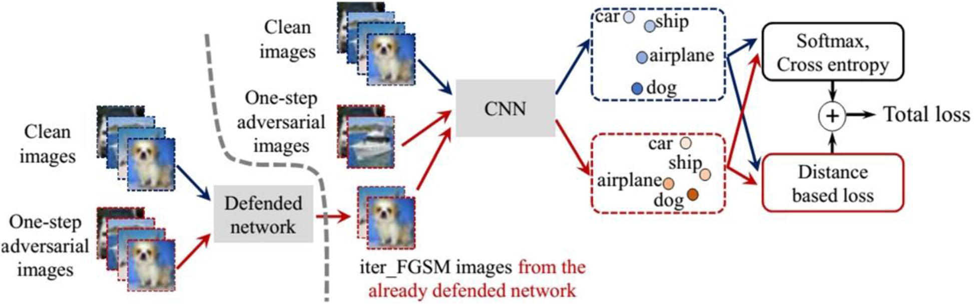
This is an interesting approach to increasing robustness. Here, we train the network by inputting adversarial images generated from an iterative defended network and one-step adversarial images from the network being trained. In addition to this, we regularize the training by penalizing the network to output very different embeddings and labels for the same samples (a clean and an adversarial sample which originally belonged to the same class as the clean, but is then perturbed), so that the convolution filters gradually learn how to ignore the pixel-level perturbations.
More methods for adversarial training and other types of defenses can be found in this paper.
An interesting observation is that training the network against these adversarial examples not only overcomes the attack by the adversary but also helps the network to generalize better. Networks trained using adversarial training are seen to perform better than their previous versions on naturally occurring test sets with no adversarial examples.
Distillation as a Defense to Adversarial Perturbations against Deep Neural Networks (Papernot et al. 2016)
Defensive Distillation is one of the prominent defense methods that have been proposed against pixel-based adversarial attacks. It uses the well-known idea of Distillation. In a way, it does not remove adversarial examples, but helps the model to generalize better and increases the chances of its perception by the human eye.
Defensive Distillation is basically the follow-up work after Papernot et al. 2016’s Jacobian approach for crafting adversarial examples, which was discussed before. We call it the Jacobian-Based-Saliency-Map (JSMA) attack. First of all, let us look at the adversarial samples crafting method that they have used in the paper. It consists of two steps -
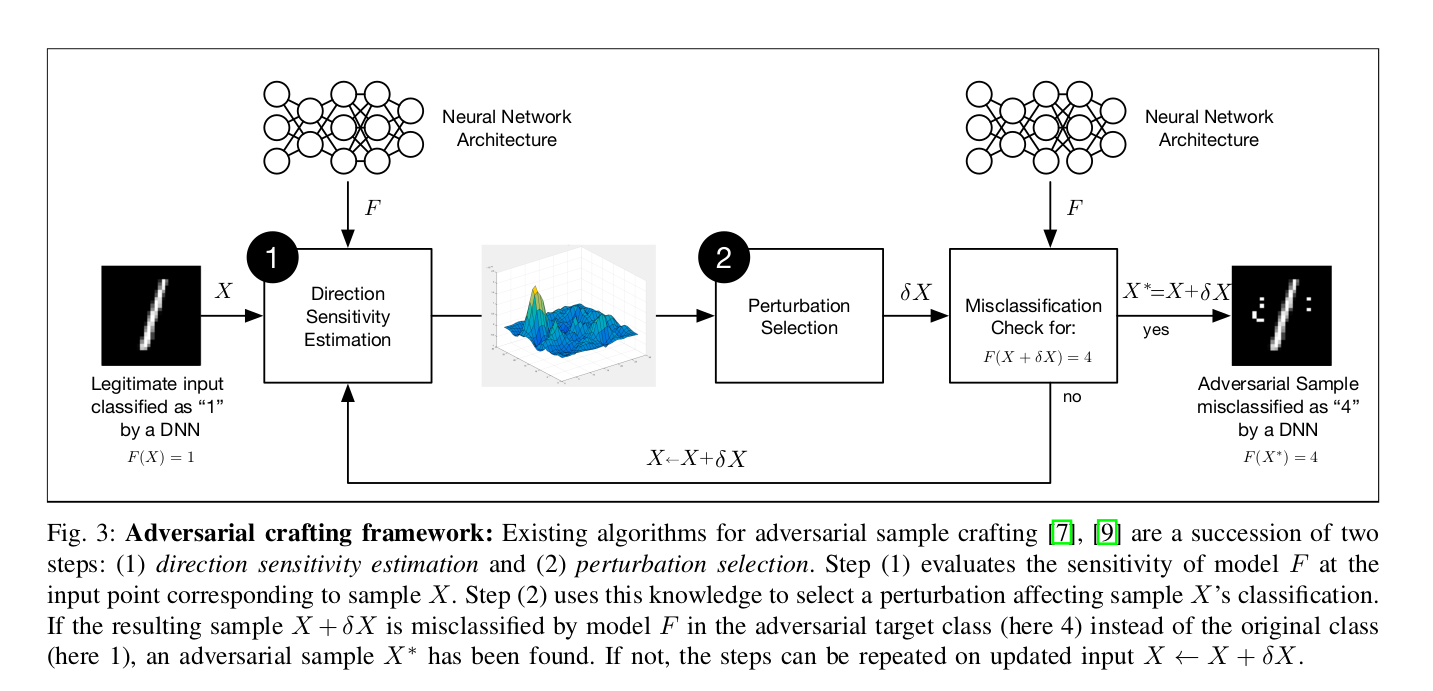
Direction Sensitivity Estimation
Here the authors estimate the sensitivity of the input pixels to a class change. The approach can be similar to the one adopted in the JSMA, i.e., using saliency maps or based on FGSM attacks introduced by Goodfellow et al. 2015
Perturbation Selection
This focuses on finding the appropriate perturbation for the pixels. Some possible approaches for this are as done in the FGSM method by changing each pixel by small amounts or in JSMA by carefully selecting sensitive pixels and attacking only those.
More on Defensive Distillation
Distillation in its original form is a training procedure enabling the deployment of Deep Neural Network (DNN) trained models in the resource-constrained devices like Smartphones. In contrast to using two neural networks, Defensive Distillation feeds the soft probability outputs from the DNN to the same network and trains it again from scratch.
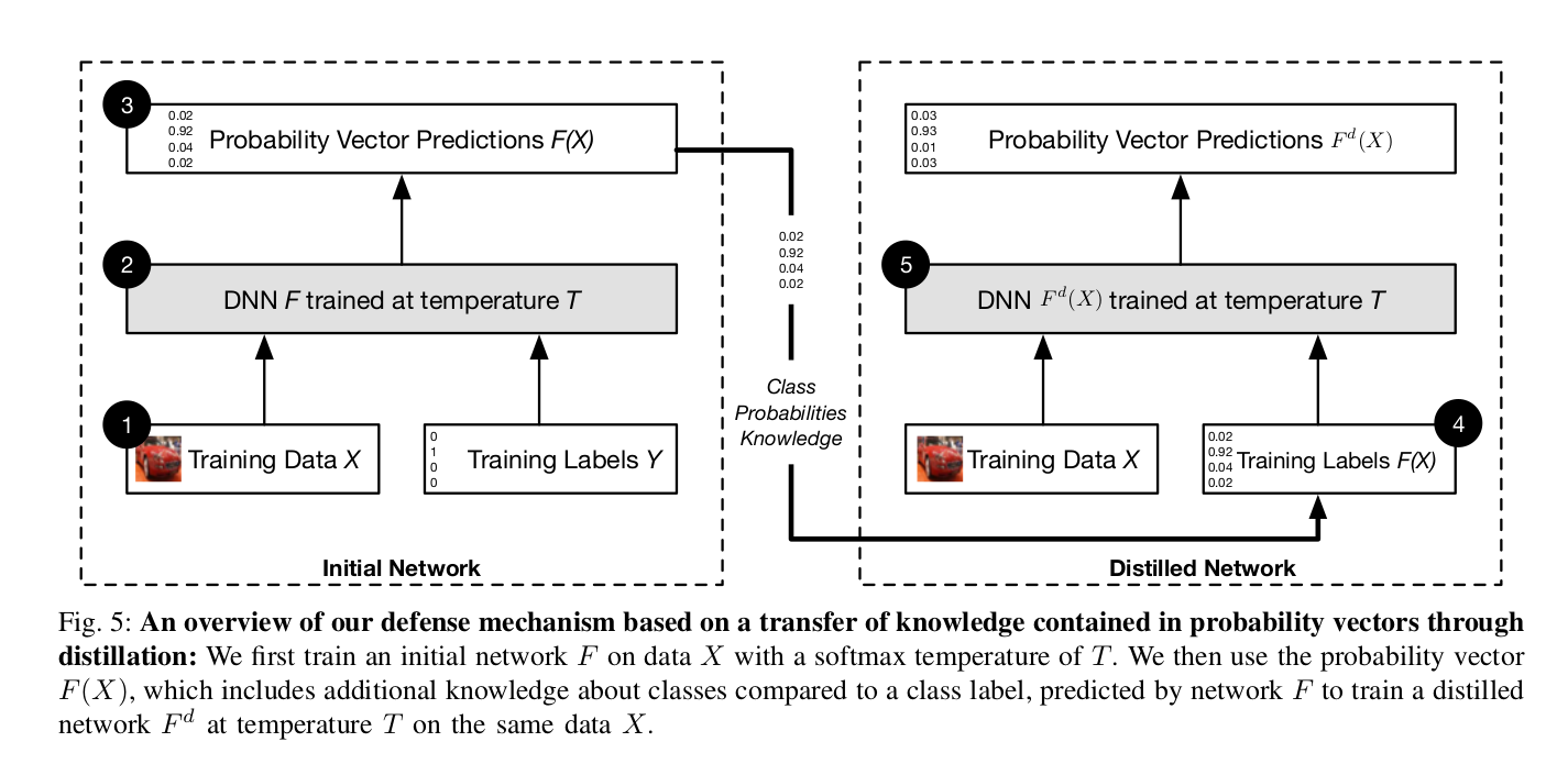
Training Procedure
First of all, the authors train the input images on a DNN at high temperature. This DNN is then evaluated on the training set at high temperature, yielding soft probabilities as outputs after the softmax layer. The DNN parameters are then reinitialized, and it is retrained with the Y-labels as the soft probability outputs from the first training procedure at high temperature. This network is then called Distilled Network and is robust to adversarial examples (robust to attacks that were introduced till then). At the test time, the temperature is again set back to 1 to get high-confidence discrete probability outputs.
In a nutshell, Defensive Distillation is a method in which a network is trained to predict the soft probabilities output by another network that was trained earlier.
Why does this tend to work?
As discussed in the paper, the intuition behind this procedure working is as follows -
Effect of High Temperature
If we compute the Jacobian of the function that the DNN tries to learn, it comes out to be inversely proportional to the temperature $T$. Hence, training the DNN at high $T$ decreases the sensitivity of the pixels to class change and, to some extent, smooths out the gradient. In other words, it smooths the model’s decision surface in adversarial directions exploited by the adversary. This makes it harder for the adversary to make the network misclassify the input by increasing the minimum required distortion.
A high temperature forces the distilled model to become more confident in its predictions.
Model now generalizes better
One of the main reasons behind the existence of adversarial examples is the lack of generalization in our models. Defensive Distillation improves on this. In the normal cases, we use the network’s output probabilities and the true hard labels to compute the cross-entropy loss for the network. This essentially reduces to computing the negative of the log of the probability corresponding to the true hard label. A necessary thing to note here is that when performing the updates, this will constrain any neuron different from the one corresponding to the true hard label to output $0$. This can result in the model making overly confident predictions in the sample class. In cases like a choice between $3$ and $8$, it is likely that the probabilities for both classes are high and close to $0.5$ (one less and other more). Just modifying a few pixels in these inputs would confuse the network and confidently predict the other wrong class.
Defensive Distillation overcomes this problem by using soft probabilities as labels in the second round. This ensures that the optimization algorithm constrains all the neurons proportionally according to their contribution to the probability distribution. This improves the generalizability of the model outside the training set by avoiding the circumstances where the model is forced to make hard predictions when the characteristics of two classes are quite similar (ex in case of $3$ and $8$, or $1$ and $7$). Hence it helps the DNN to capture the structural similarities between two very similar classes.
Another explanation is that by training the network with the soft labels obtained from the first round, we avoid overfitting the actual training data. However, this does not tend to work if we consider the linearity hypothesis for adversarial examples as proposed by Goodfellow et al. 2015
As a keynote, when Defensive Distillation was introduced, it failed all the attacks that existed till then! However, one year later, the stronger Carlini-Wagner attack was introduced, which Defensive Distillation was not able to counter. It is discussed below.
Looking at Carlini-Wargner attack - Breaking Defensive Distillation!!
Towards Evaluating the Robustness of Neural Networks(Carlini et al. 2017)
Introduction and Problem formulation
I would like to discuss this method in much more detail, as the points highlighted in the paper force us to think about defensive distillation from another perspective and show how easy it can be to break the networks (with seemingly no visual difference), even on the instances where the prior methods struggle to find adversarial examples with minimal perturbation.
The objective of this paper is to address the following question -
\[\begin{align}&\text{How should we evaluate the effectiveness of defenses against adversarial attacks?} \\ \\ &\text{or in other words -} \\ \\ &\text{How can one evaluate the robustness of a Neural Network?}\end{align}\]Note: Feel free to go back to the definition of Robustness discussed earlier.
There are generally two approaches for this -
-
Construct proofs for a lower bound on the robustness. This means to ensure that the network will at least perform as good as some lower limit. In the context of images, this corresponds to giving some guarantee that if the input is perturbed at most by some amount, the output will still be classified correctly.
-
Demonstrate attacks for an upper bound on the robustness. This corresponds to introducing an attack that successfully breaks a defense system, thereby putting an upper bound on the performance.
Coming up with the proofs for the first method is difficult. Many times, it might be easier to come up with strong attacks and use them as benchmarks for evaluation. This paper does the same - It breaks defensive distillation by the second approach.
The attack method introduced in this paper is perhaps the strongest of all we discussed before. The Carlini-Wagner attack is the first to generate adversarial examples for ImageNet. All the other attack methods fail to produce “neat” adversarial examples either due to the maximum limiting perturbation allowed or computational expense. This method even works against Defensive Distillation, while all the other attacks discussed above fail, getting their success rate decreased from $95\%$ to $0.5\%$. However, this attack gets a success rate of $100\%$ on distilled as well as undistilled Neural Nets!
Carlini-Wagner gives three forms of the attack, differing in the $L_p$ norms, which measure the distance between pixels -
-
$L_0$ distance corresponds to the number of pixels that have been altered in the image.
-
$L_2$ corresponds to the Euclidean distance between the images - squaring all the pixel-values, summing, and taking the square root.
-
$L_\infty$ measures the maximum difference between any two pixels in the images. Informally, it means that no pixel is allowed to change beyond an upper limit.
Now, following is the optimization problem that we want to solve -
\[\min_{\delta} D(x, x+\delta)\] \[\text{such that} \; C(x+\delta) = t,\] \[\text{and }x+n \; \epsilon \; [0, 1]^n\]It means for an input image $x$, find a perturbation $\delta$ such that it minimizes $D$, as measured by an $L_p$ norm metric (three of them discussed above). This is subject to that the network/classifier $C$ classifies the perturbed image into the target class $t$, and the perturbed pixel still lies in the valid range (0 and 1 correspond to 0 and 255 normalized pixel-values respectively). The first condition lets source-target misclassification, and the second makes sure that the image is still valid with respect to the input distribution.
Let us divide the optimization problem into three parts -
I. The first constraint $C(x+\delta)=t$ is highly non-linear. So we do a modification by introducing an objective function $f$ such that -
\[C(x+\delta)=t \text{ if and only if } f(x+\delta)\leq0\]The paper gives many possible objective functions, but we’ll see the one that works the best according to them -
\[f=max(max[Z(x\prime)_{i}: i \neq t] - Z(x\prime)_{t}, 0)\]Here $Z$ are the output logits of the network.
II. Now, instead of using the constraint version -
\[\min_{\delta} D(x, x+\delta)\] \[\text{such that} \; f(x+\delta)\leq0,\] \[\text{and }x+n \; \epsilon \; [0, 1]^n\]we use an alternative version -
\[\min_{\delta} D(x, x+\delta) + c \cdot f(x+\delta)\] \[\text{such that } x+n \; \epsilon \; [0, 1]^n\]III. For the second constraint, we use a change of variables such that the image still remains valid. We introduce a new variable $w$ and instead of optimizing over $\delta$, we optimize over $w$.
\[\delta_i = 0.5(\tanh(w_i)+1)-x_i\]Now, $-1\leq\tanh(w_i)\leq1$, which implies $0\leq x+\delta_i\leq1$. Hence the solution remains the same.
Summing altogether, the optimization problem for $L_2$ attack is -
\[\min_{w} [\lVert0.5(\tanh(w)+1)-x\rVert^2_2 + c \cdot f(0.5(\tanh(w)+1))]\] \[\text{where } f(x\prime)=max(max[Z(x\prime)_{i}: i \neq t] - Z(x\prime)_{t}, -\kappa)\]The left term in the minimization objective denotes the similarity function between the original and perturbed samples, with the distance measured in $L_2$ norm. The right term in the objective function ensures the first condition ($f$ is negative or $0$ if the target class is $t$). The second condition is satisfied implicitly by the change of variables (due to the range of $\tanh$). The constant $\kappa$ is a tuning parameter denoting the confidence with which the input is misclassified. If its magnitude is large, the output logits for class $t$ should be large as compared to the output logits of all other classes, thereby forcing the network to find an adversarial example with higher confidence. Metaphorically, the first term denotes distance, and the second term denotes confidence.
Finally, the whole objective minimizes the distortion, simultaneously misclassifying the original input to some target class. The trade-off between the two parts of the objective is steered by the constant $c$. Now, how to choose $c$?
If $c$ is large, gradient descent (or modified Adam updates) takes steps in an overly-greedy manner forcing the whole minimization procedure dominated by the second term and ignoring the distance loss function. This would lead to the adversarial example being too different from the original one and hence sub-optimal solutions. However, if $c$ is very small (close to $0$), gradient descent would not be able to make any progress, and we won’t find any adversarial examples. For a fixed constant $c$ to be useful, it is important that the two terms in the objective ($D$ and $f$) should remain approximately equal. So we use a modified binary search for finding the suitable $c$. We start with a small $c$ value, say $0.01$, plug it into the objective, and run $10,000$ steps of gradient descent with Adam optimizer to find the adversarial example. Repeating this process by doubling the value of $c$, we get the following curve -
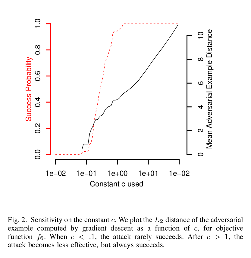
The curve is plotted by evaluation on the MNIST dataset. The x-axis in the above figure represents $c$ plotted on the log-scale. The left y-axis shows the probability with which we can generate adversarial examples, and the right one shows the mean adversarial example distance (left term in the objective). Note that the mean distance increases as $c$ increases, as expected.
Here we can see that at $c=1$, we can find an adversarial example with $100\%$ probability and minimum possible distortion. Higher values of $c$ yield adversarial examples with the same maximum probability, but the distortion increases.
Discretization post-processing
This is an important step in the evaluation of this attack. Note that we take the pixel intensities in the range $[0, 1]$. However, in a valid image, each pixel intensity must be a discrete integer between $0$ and $255$, both inclusive. This additional constraint is not captured in the formulation we saw above. The reason is that the intensity is rounded-off to the nearest integer, and we get $\lfloor 255(x_i+\delta_i) \rfloor$ (assuming rounding-off to lower value). Doing so degrades the quality of the attack. However, this is not true for the weaker attacks that we discussed before. For instance, in FGSM, discretization rarely affects the quality of the attack. However, in the C-W attack, the perturbations to the pixels are so small that discretization effects cannot be ignored.
Hence after finding an adversarial example by optimizing the objective function, we perform a greedy search on the lattice defined by the discrete solutions by changing one pixel-intensity at a time. All the results in the paper include this post-processing step.
The three attacks
$L_2$ attack
This uses the $L_2$ metric in the objective function. The optimization problem formulation is already highlighted before -
\[\min_{w} [\lVert0.5(\tanh(w)+1)-x\rVert^2_2 + c \cdot f(0.5(\tanh(w)+1))]\] \[\text{where } f(x\prime)=max(max[Z(x\prime)_{i}: i \neq t] - Z(x\prime)_{t}, -\kappa)\]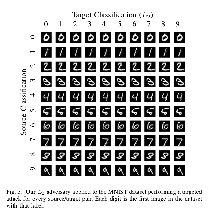
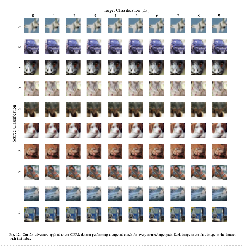
This shows the $L_2$ attack on the MNIST and CIFAR10 dataset. In MNIST, the only case where one would find a little visual difference between the original and the adversarial digit is when the source is $7$, and the target is $6$. For CIFAR10, there is no visual distinction from the baseline image.
The other two norms are not straight-forward as $L_2$ and require some bells and whistles to work.
$L_0$ attack
The $L_0$ metric is non-differentiable, hence cannot be used directly for gradient descent procedure. $L_0$ measure the distance in terms of the number of pixels that have different intensities in the two examples. Hence we use a shrinking iterative algorithm that starts from the whole set of pixels that could be modified, makes an $L_2$ attack on the input image, and then freezes the pixels modifying, which affects the output by less than some specified amount. This is then repeated until we find a minimal set of pixels, and perturbing, which will change the output class the most.
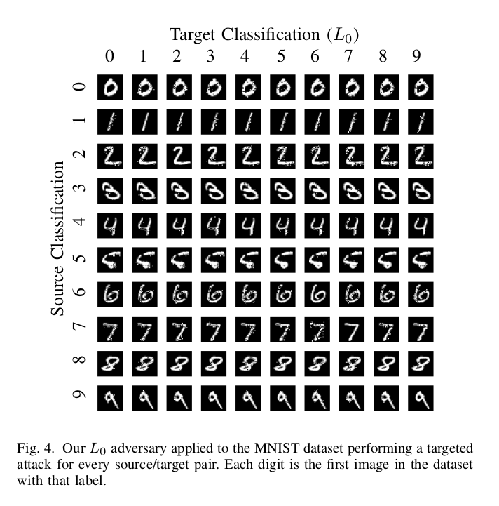
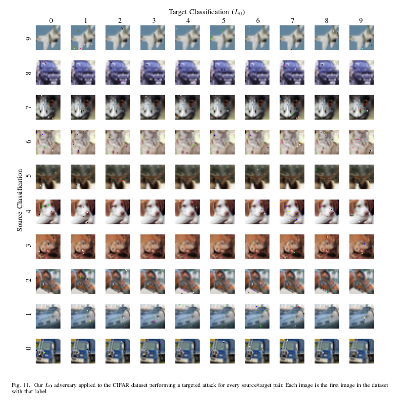
As we can see, for MNIST, this method produces images with more distortions as compared to the $L_2$, but still, the adversarial examples are not so different. The result is the same as the previous for CIFAR10.
$L_{\infty}$ attack
This distance metric is not fully differentiable at many places, and standard gradient descent does not perform work well if we naively optimize the following -
\[\min_{\delta} [\lVert\delta\rVert_{\infty} + c \cdot f(x+\delta)]\]This is because of the following - $\lVert\delta\rVert_{\infty}$ penalizes only the largest absolute value in all of the pixels. Now, say we have two pixels having intensities $\delta_i=0.5$ and $\delta_j=0.5-\epsilon$, where $\epsilon$ is very small. Using this norm penalizes only $\delta_i$ and not $\delta_j$, even though $\delta_j$ is already large (the derivative of $\lVert\delta\rVert_{\infty}$ with respect to $\delta_j$ is $0$). Suppose at the next iteration, the pixel-values become $\delta_i=0.5-\epsilon\prime$ and $\delta_i=0.5+\epsilon\prime\prime$. This is start a mirror image of the process that happened before. In this way, gradient descent will keep oscillating around $\delta_i=\delta_j=0.5$, making almost no progress.
To get around this, we use the following iterative attack -
\[\min_{\delta} [\sum_i[max((\delta_i-\tau), 0)] + c \cdot f(x+\delta)]\]Here, all the pixels having intensities more than $\tau$ are penalized. This prevents oscillations as all the large values are penalized.

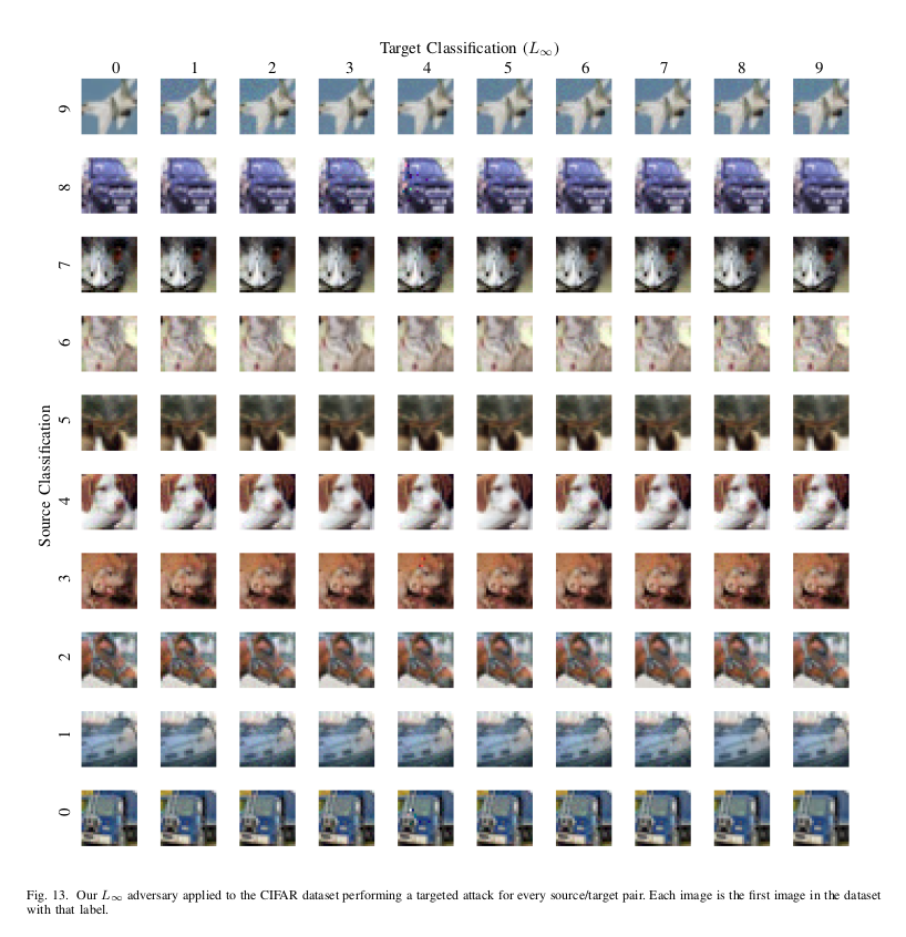
The perturbations are noticeable on the MNIST dataset, but still are recognizable as their original classes. Attack on CIFAR10 has no visual difference from the baseline input. On the ImageNet dataset, $L_{\infty}$ attack produces such small perturbations that it is possible to change the classification of the input into any desirable class by changing just the lowest bit of each pixel, a change that would be impossible to detect visually.
It is interesting to note that in all the three attacks on MNIST,
the worst-case distortion is when source class in 7 and target class in 6.
Attack evaluations also show that as the learning task becomes more difficult, other methods produce a worse result, while the C-W attack performs even better.
Generating Synthetic digits
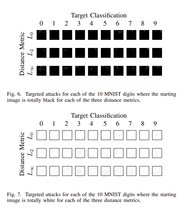
This is an interesting experiment carried out to show the strength of this attack. We start from a completely black or white image and apply the three distance metrics to successfully classify the image in each of the ten target classes. We can see the amount of perturbation required to misclassify the blank images to any target class is almost negligible! Here all the black images were initially classified as $1$ and all the white images as $8$, hence they require no change.
A similar experiment is carried out by Papernot et al. 2016. However, with their attack, one can easily recognize the target digit for classes $0$, $2$, $3$, and $5$.
Evaluating Defensive Distillation
As shown in the paper, these attacks have a success rate of $100\%$, even for defensively distilled networks. Distillation adds almost no value over the undistilled networks - $L_0$ and $L_2$ attacks perform slightly worse, and $L_{\infty}$ performs approximately the same.
Following are some key points in the paper which explain the failure of Defensive Distillation -
”””
The key insight here is that by training to match the first network, we will hopefully avoid overfitting against any of the training data. If the reason that neural networks exist is that neural networks are highly non-linear and have “blind spots” [46] where adversarial examples lie, then preventing this type of over-fitting might remove those blind spots.
In fact, as we will see later, defensive distillation does not remove adversarial examples. One potential reason this may occur is that others [11] have argued the reason adversarial examples exist is not due to blind spots in a highly non-linear neural network, but due only to the locally-linear nature of neural networks. This so-called linearity hypothesis appears to be true [47], and under this explanation, it is perhaps less surprising that distillation does not increase the robustness of neural networks.
”””
We can prove empirically that distillation does not increase the robustness of the networks. In the previous works, it was found that increasing the temperature consistently reduces the attack rate. On MNIST, the success rate goes from $91\%$ at $T=1$ to $24\%$ at $T=5$ and finally $0.5\%$ at $T=100$. However, this is not true with C-W attacks -
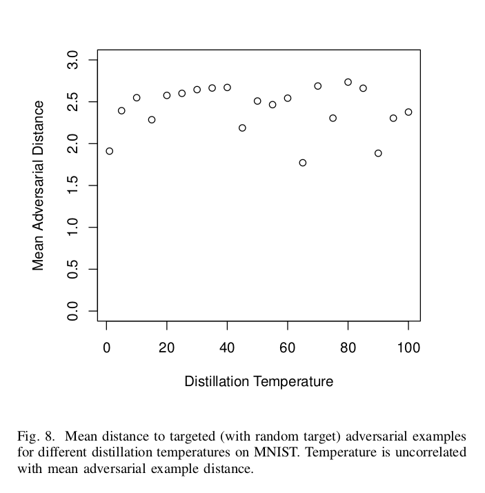
Here we see that there is no positive correlation between the distillation temperature and the mean adversarial distance (as observed in the weaker attacks). Note that the latter measures the robustness of the networks (expected value of the radius is the mean adversarial distance). In fact, the correlation coefficient is negative. This suggests that increasing the temperature does not increase the robustness; instead, it only causes the previous weaker attacks to fail more often.
Breaking Defensive Distillation again with Transferability!
We demonstrated that the C-W attack successfully works against the distilled network. But can it be that an adversarial example created from an undistilled network fails (or transfers to) a distilled network? YES!!
Recall that this is the Transferability property of adversarial examples, as discussed in Szegdey et al. 2014. This is achieved by generating high-confidence adversarial examples on a standard model. Remember the constant $\kappa$ in the objective function?
\[f(x\prime)=max(max[Z(x\prime)_{i}: i \neq t] - Z(x\prime)_{t}, -\kappa)\]Increasing this $\kappa$ value forces the network to find adversarial examples with higher-confidence. What is means is that the adversarial example should not barely cross the boundary and enter into the target class (or another random class in case of untargeted attacks); instead it should be classified to the target class with high probability.
There are two experiments for testing this hypothesis -
I. Transferring to a standard model
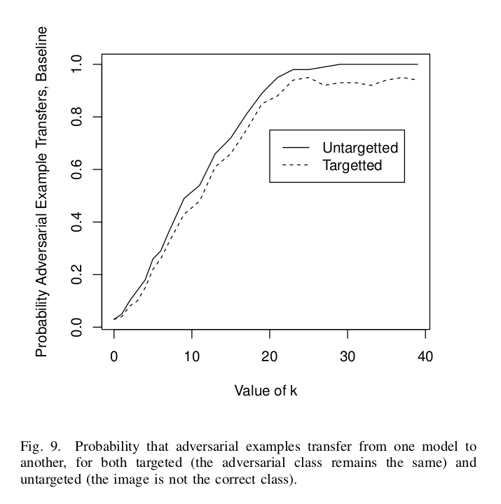
In this experiment, we divide the MNIST dataset into two parts and train two separate standard networks on them. Adversarial examples that break the first network are generated with an increasing value of $\kappa$. We can see the results for both Untargeted as well as Targeted scenarios.
Note that the probability increases almost linearly from $\kappa = 0$ to $20$ till it becomes 1. It remains constant for higher values of $\kappa$.
II. Transferring to a distilled model
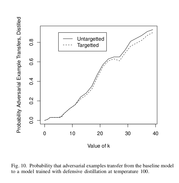
The setup here is the same as the previous, with a difference that now that the second model is trained using Defensive Distillation. Again, we find that adversarial examples do transfer. Interestingly, here the probability reaches $1$ at $\kappa = 40$.
Conclusion
Finally, this work tells us how easy it can be to fail powerful models, not only in Deep Learning but in all of Machine Learning. And this can be possible with extremely minute perturbations, as we saw, which are almost undetectable to the human eye (or least the distortion is not so much that it would be classified incorrectly by humans). The attacker need not even have complete access to the network. It can generate adversarial examples on its own network and use then on the victim network. Thanks to Transferability :P.
This work also suggests that even though Defensive Distillation can block the flow of gradients, it is not immune to stronger attacks, like the ones discussed here. Hence while proposing a defense system or before deploying models, we should take care of three things -
-
The defense system should increase the robustness of the model, as measured by the mean adversarial distance.
-
It should break the Transferability property. Otherwise, it would be easy for attackers to generate adversarial examples on their own models.
-
It should successfully beat stronger attacks like the Carlini-Wagner attacks introduced here.
Back to discussing defenses
Defense-GAN: Protecting Classifiers Against Adversarial Attacks Using Generative Models (Samangouei et al. 2018)
This is a Generative model-based strategy for preventing the attacks. It does not make the network more robust; instead, it uses Generative Adversarial Nets (GANs) to introduce a pre-processing step which removes the adversarial perturbations, making the example cleaner.
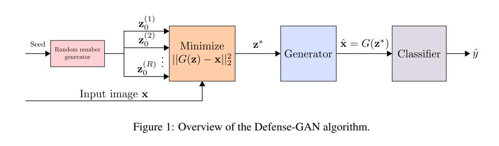
This technique is applicable to combat both white-box and black-box adversarial attacks against classification networks. At the inference time, when the attacks happen, prior to feeding an image $x$ to the network, we project it onto the range of the Generator by minimizing the reconstruction error $\lVert G(z)-x\rVert^2_2$. Since the Generator was trained to model the unperturbed training data distribution, this added step results in a substantial reduction of any potential adversarial noise. The minimized $z$ is then given as input to the Generator, which generates an image $G(z)$, which is then given to the actual classifier.
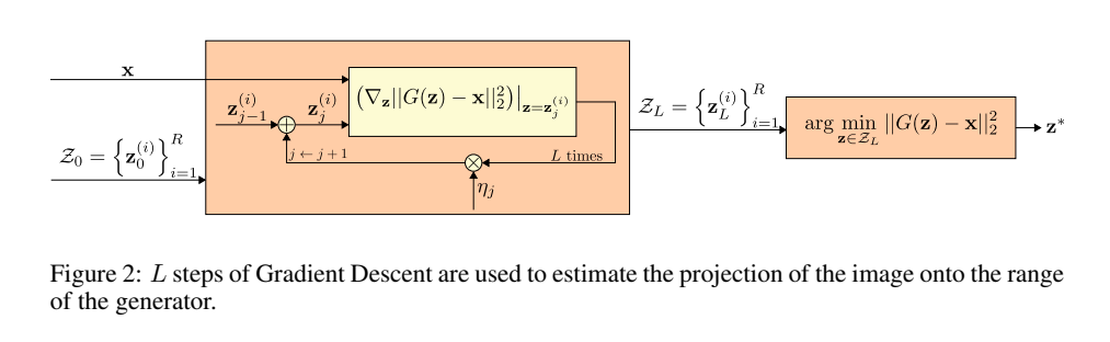
The minimization problem above is highly non-convex. Hence the optimal value of $z$ is approximated via $L$ steps of Gradient Descent using $R$ different random initializations of $z$, as shown in the above figure.
Compared to the defenses introduced before, this method differs in the following ways (as shown in the paper) -
-
Defense-GAN can be used in conjunction with any classifier as it does not modify the classifier structure itself. It can be seen as an add-on or pre-processing step prior to classification.
-
Defense-GAN can be used as a defense to any attack: it does not assume an attack model, but simply leverages the generative power of GANs to reconstruct adversarial examples.
-
If the GAN is representative enough, retraining the classifier should not be necessary, and any drop in performance due to the addition of Defense-GAN should not be significant.
-
Defense-GAN is highly non-linear, and white-box gradient-based attacks will be difficult to perform due to the Gradient Descent loop.
End thoughts
Having seen these attack approaches, a nice explanation of the existence of such attacks (especially the pixel-based ones) is given by the story of Cleverhans -
”””
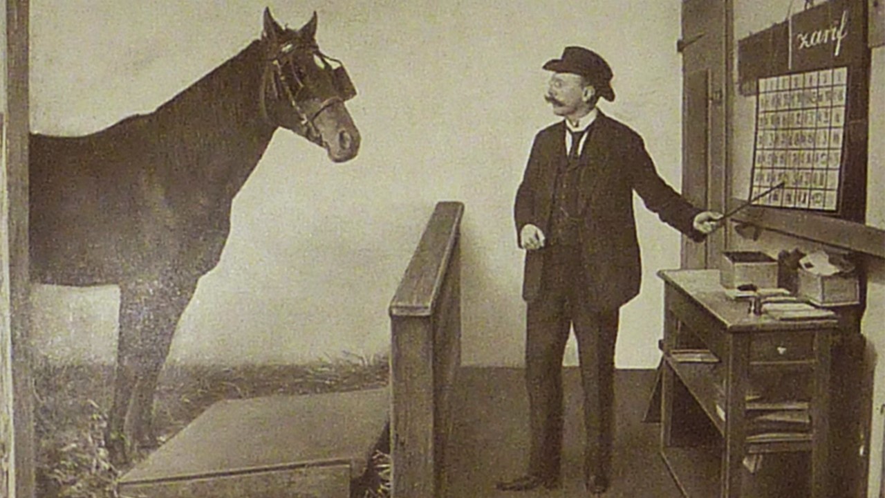
So Cleverhans was a horse, and its owner had trained it to solve arithmetic problems. The owner would say, “Cleverhans, what is 1+1?”, and it would tap its feet two times, and the crowd would cheer for him, or its owner would give it some fruit to eat as a reward. However, a psychologist examined the situation and figured out that the horse did not actually learn to do arithmetic. He discovered that if the horse was placed in a dark room with no audience and a person wearing a mask would ask the arithmetic problem; it would just continue to tap feet on the floor waiting to receive some signal to stop.
”””
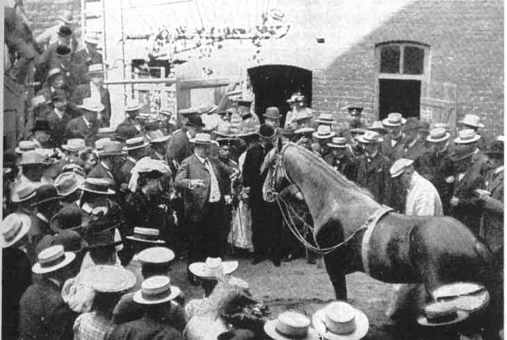
This is exactly what is happening with our Machine Learning models. They fit the training and the test set with very high accuracies, but if an adversary intentionally designs some example to fail them, they get fooled. Goodfellow et al. 2017 view adversarial examples broadly as – Inputs to Machine Learning models that an attacker has intentionally designed to cause the model to make a mistake. In the story of Cleverhans, the horse assumed the correct signal to be the cheerings of the crowd or the fruit that its owner would give when it reached the correct number of taps. This is similar to a Weather predicting ML model. Instead of knowing that the clouds actually cause rains, it believes that the “presence” of clouds causes rains.
There is a small difference between the two things, but it is this difference that only fools our ML models. These models associate the occurrence of events but do not know what actually caused them.
It is not that our models do not generalize to test sets. Like in the story of Cleverhans, the model (horse) did generalize to solving the problem correctly in front of the crowd, which indeed is a naturally occurring test set. But it did not generalize to the case when the adversary specifically creates a test case to fail it (worst-case scenario). More importantly, this test example need not be off the distribution. Like in the story, the scenario created by the psychologist is totally legitimate. Similarly, these adversarial examples are also valid test cases for the model.
Also, it is not that these adversarial examples are a characteristic property of Deep Learning or Neural Networks. The linear nature of our ML models (linear or piecewise linear with respect to the input) is problematic, and because Neural Networks build upon their architecture, they inherit this flaw. Ease of optimization in our models has come at the cost of these intrinsically flawed models that can be easily fooled.
These arguments generalize to both types of attacks we have discussed. In pixel-based attacks, we are able to find adversarial examples that look absolutely legit but still confuse the network. In the adversarial policy attack too, the victim policies were used to seeing certain naturally occurring opponents (test cases) where say in You shall not pass, the opponents would try to push the victim in some way to prevent crossing the line. However, the adversaries fooled the victim by adjusting themselves into unconventional positions, in which a human would be easily able to win. This leaves us with the following question -
Are we really close to human-level General Machine Intelligence?
References and Further reading (non-exhaustive)
Deep Neural Networks are easily fooled: High confidence predictions for unrecognizable images
DeepFool: a simple and accurate method to fool deep neural networks
CopyCAT: Taking Control of Neural Policies with Constant Attacks
Stealthy and Efficient Adversarial Attacks against Deep Reinforcement Learning
Targetted Attacks on Deep Reinforcement Learning Agents through Adversarial Observations
Following paper gives a collection of most of the attacks and defenses introduced till now -