Temporal Difference Learning
In this article, we will learn about Temporal Difference (TD) learning, a value-based method for solving Reinforcement Learning problems. We will also implement Tabular TD algorithms from scratch on Gridworld and Cliff-walking environments.
TD-learning: A brief Introduction
While sampling-based methods like Monte-Carlo (MC) prove to be advantageous over Dynamic Programming (DP) algorithms, a significant problem associated with them is that we have to wait for the episode to end (they are not online). The discounted sum of rewards till the end of the episode ($G_t$) is used as the target value in the Value-function updates. However, this may take a lot of time if the episode is lengthy, or forever in case of non-episodic tasks. So what is the solution to this?
\[G_t = R_{t+1} + \gamma R_{t+2} + \gamma^2 R_{t+3} + ... + \gamma^{T-t-1} R_T\]One option might be to truncate the return and end the episode after a certain number of threshold time-steps. However, this might reuslt in the loss of information, especially in the sparse and delayed reward domains, where the agent gets rewards only after trying out many actions in a proper sequence, instead of randomly wandering around. To get over this, Dynamic Programming already provides a way to tackle this problem in the form of bootstrapping (updating the value estimate for a state from the estimated values of subsequent states). So instead of waiting till the end of the episode, we consider the true discounted reward values up to a particular time step and then take the discounted estimated value function for the next state. So why not combine these two approaches.
We use Temporal-Difference for this. The idea is very simple and elegant. Let me describe it with an example - Assume that an agent is playing the game of Tic-Tac-Toe against some fixed opponent. Keeping the opponent fixed reduces the problem to a single-agent MDP instead of Multi-agent. The agent does not have any information about the environment and just gets a reward signal $+1$ and $-1$ at the end of a game if it wins or otherwise, respectively. In this setting suppose the agent thinks that from the current state $s_t$, on taking some particular action $a_t$, it will have $0.9$ probability of winning. It executes that state-action pair and goes into the future and observes the value of the next state. However, suppose the agent had played a bad move which ended up in it losing the game in the future. Clearly, the agent had not anticipated this. So it comes back to that state-action pair $s_t, a_t$ and corrects its estimation of the probability of winning the game by reducing it from $0.9$ to say $0.7$. This is exactly the idea of Temporal-Difference! You play some move, see its outcome based on the estimation of the future states, and then come back to correct your current estimation. Note that vice-versa would happen if the agent had won the game, and it would then try to increase the probability of winning from that state-action pair.
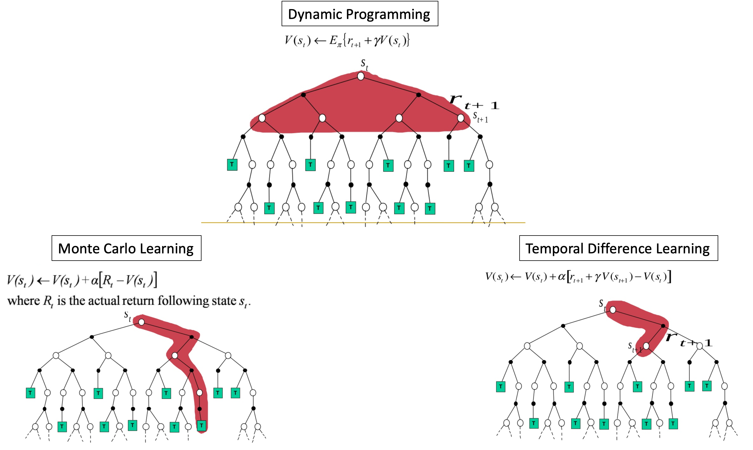
Temporal Difference (TD) learning is a family of model-free methods that combines the sampling nature of Monte-Carlo with the bootstrapping behavior of DP. Model-free means that we need not know the details of the environment like the transition and reward probabilities from one state to another given an action. They can be implemented in an online-incremental fashion, making them suitable even for continuing tasks. The figure shows a comparison between the three methods for value-based learning.
To be precise, the method that we are going to discuss is TD(0), where the 0 indicates the extent of bootstrap. It means that we take the true value of just the immediate reward and then the discounted value for the VF for the next state. A more general version TD($\lambda$) is shown below.
\[G_{t:t+n} = R_{t+1} + \gamma R_{t+2} + \gamma^2 R_{t+3} + ... + \gamma^{n-1} R_{t+n} + \gamma^n V_{t+n-1}(S_{t+n})\]Note that this is Forward-view TD($\lambda$). The more efficient and practical Backward-view TD($\lambda$) is implemented using Eligibility Traces.
Fun Fact:
One of the major contrasting features between MC and TD learning is that TD learning is
more suited for Markovian environments, making it a better choice for many Markovian RL
problems!
The intuition behind this is that MC methods estimate the value functions, which minimize the mean-squared training error. It means that the values estimated by MC are closest possible to the actual returns observed during training, which is evident since we wait for the episode to terminate while making updates. On the other hand, TD learning converges to the maximum likelihood Markov model, by implicitly building an MDP to describe the environment and which best fits the data. So it first fits an MDP and then solves it, which helps it in exploiting the Markov property. So instead of looking at complete trajectories (as we did in MC), we can understand the environment in terms of states. The current state completely summarizes all the information in the past, which is required to take an optimal action. Hence, in Markovian environments, bootstrapping would help, and we need not necessarily see the actual returns.
Moving on, in general Reinforcement Learning, the problems are broadly divided into Prediction and Control. The prediction problem aims at finding the optimal value function, given a policy, while the control methods find optimal value function as well as optimal policy.
TD-Prediction
The Prediction problem involves sampling an action using the given policy and making updates for the value function in the direction of the error between the predicted value (target) and the old estimate.
\[V(S_t) := V(S_t) + \alpha [ R_{t+1} + \gamma V(S_{t+1}) - V(S_t) ]\]The error is weighed by a step-size parameter $\alpha$ (learning rate), which indicates the extent to which the new information about the current state ($R_{t+1} + \gamma V(S_{t+1})$) updates our current estimate. This is because the new information available to us tells a bit more about the environment (since we have seen one step of the actual environment). $\alpha$ = 0 indicates that the old estimate is retained, while $\alpha$ = 1 represents completely forgetting the previous estimate and using the new one. There can be some issues of convergence with probability 1 using a constant step-size since it does not obey the conditions for stochastic approximation, as shown below.
\(\displaystyle \sum_{n=1}^\infty \alpha_n = \infty,\) \(\displaystyle \sum_{n=1}^\infty \alpha^2_n = \infty\)
Nevertheless, it is guaranteed to converge in the mean case.
The discount factor $\gamma$ tells how much we care about the delayed rewards. $\gamma$ = 0 indicates myopic nature of caring just about the immediate reward $R_{t+1}$, while $\gamma$ = 1 indicates we care about the distant rewards as well.
Setting up the environment
Let us start by defining our environment. We consider a $5\times7$ Gridworld and test the code for a Uniform Random policy and a Deterministic, greedy optimal policy. The environment consists of 2 Terminal states $T$, and the goal is to learn the value function for a given policy for all the states in the space. The rewards are defined as shown in the code.
Let us write the code for this environment.
'''
####################### SMALL GRIDWORLD ###########################
    GridWorld like:

    T o o ..........o
    o o o ..........o
    . .             .
    . .             .
    . .             o
    . .             o
    o o o ......o o T
Actions:
    UP (0)
    DOWN (1)
    RIGHT (2)
    LEFT (3)

Rewards:
     0 for going in Terminal state
    -1 for all other actions in any state

Note: State remains the same on going out of the maze (but -1 reward is given)
'''
def env(state, action):
    # return_val = [prob, next state, reward, isdone]
    num_states = rows * columns
    isdone = lambda state: state == 0 or state == (num_states-1)
    reward = lambda state: 0 if isdone(state) else -1

    if(isdone(state)):
        next_state = state
    else:
        if(action == 0):
            next_state = state - columns if state - columns >= 0 else state
        elif(action == 1):
            next_state = state + columns if state + columns < num_states else state
        elif(action == 2):
            next_state = state + 1 if (state + 1) % columns else state
        elif(action == 3):
            next_state = state - 1 if state % columns else state
    # State Transition Probability is 1 because the environment is deterministic
    return_val = [1, next_state, reward(state), isdone(next_state)]
    return return_val
Setting the Hyperparameters
alpha = 0.1 # Learning Rate
rows = 5
columns = 7
num_states = rows * columns
num_actions = 4
gamma = 0.999 # Discount Factor
episodes = 100000 # Number of games played
# UNIFORM RANDOM POLICY
rand_policy = np.ones((num_states, num_actions))/num_actions
# GREEDY DETERMINISTIC POLICY
deter_policy = [[1, 0, 0, 0],[0, 0, 0, 1],[0, 0, 0, 1],[0, 0, 0, 1],[0, 0, 0, 1],[0, 1, 0, 0],[0, 1, 0, 0],
                [1, 0, 0, 0],[1, 0, 0, 0],[1, 0, 0, 0],[1, 0, 0, 0],[1, 0, 0, 0],[0, 1, 0, 0],[0, 1, 0, 0],
                [1, 0, 0, 0],[1, 0, 0, 0],[1, 0, 0, 0],[1, 0, 0, 0],[0, 1, 0, 0],[0, 1, 0, 0],[0, 1, 0, 0],
                [1, 0, 0, 0],[1, 0, 0, 0],[1, 0, 0, 0],[0, 1, 0, 0],[0, 1, 0, 0],[0, 1, 0, 0],[0, 1, 0, 0],
                [1, 0, 0, 0],[1, 0, 0, 0],[0, 0, 1, 0],[0, 0, 1, 0],[0, 0, 1, 0],[0, 0, 1, 0],[1, 0, 0, 0]]
Code for the algorithm
def td_pred(policy, flag):
    # Initialize Value function
    VF = np.zeros(num_states)
    for episode in range(episodes):
        # Initialize S
        curr_state = np.random.randint(0, num_states)
        while True:
            # Sample an action from S
            # flag indicates the policy taken into account
            curr_action = np.argmax(policy[curr_state]) if flag else np.random.randint(0, num_actions)
            # prob: State Transition Probability
            # reward, next_state: Immediate reward and next state on taking curr_action in curr_state
            # isdone: Whether the next state is Terminal or not
            prob, next_state, reward, isdone = env(curr_state, curr_action)
            # Update the current state value
            VF[curr_state] = VF[curr_state] + alpha * (reward + gamma * VF[next_state] - VF[curr_state])
            curr_state = next_state
            if isdone:
                break
    return VF
Analyzing the output
For Uniform Random policy
#Value Function for Uniform Random policy:
 [[  0.         -22.8145219  -41.04389241 -49.63242096 -53.92961483 -55.14102473 -53.66020676]
  [-33.77022359 -40.97067518 -45.58716647 -52.03257216 -53.19503964 -53.81359137 -50.4964524 ]
  [-45.93384504 -47.98148611 -53.73653323 -53.05661863 -50.92048008 -43.9545928  -40.13167269]
  [-54.48416843 -55.81282363 -56.54764755 -53.70269288 -44.73549628 -33.37134078 -21.46056466]
  [-60.74101434 -58.86750144 -57.60923797 -54.66034268 -43.67117606 -28.48519834   0.        ]]
The output shows the estimated value function for each of the states for the given policy.
For Greedy policy
#Value Function for deterministic greedy policy:
[[ 0.       -1.       -1.999    -2.997001 -3.994004 -4.99001  -3.994004]
 [-1.       -1.999    -2.997001 -3.994004 -4.99001  -3.994004 -2.997001]
 [-1.999    -2.997001 -3.994004 -4.99001  -3.994004 -2.997001 -1.999   ]
 [-2.997001 -3.994004 -4.99001  -3.994004 -2.997001 -1.999    -1.      ]
 [-3.994004 -4.99001  -3.994004 -2.997001 -1.999    -1.        0.      ]]
As expected, the output shows the values for the shortest and optimal path from each state to terminal state.
TD-Control
The Control problem requires us to find both the optimal policy as well as value function. Here comes the dilemma of Exploration v/s Exploitation. This is one of the most fundamental problems in RL, and various approaches have been proposed over the years to strike a good balance between the two. The agent needs to make full use of information about the environment available to gain the maximum reward. Still, for knowing more about the environment, it needs to explore, which might come at the cost of getting less reward. As one would observe, it is a fundamental trade-off.
Broadly, there are two approaches to balance exploration and exploitation-
On-policy TD-Control (SARSA)
On-policy is what till now we have been following where the policy that is used to make decisions (sample the actions) is the same as one used for evaluation and improvement. For on-policy control, we use a strategy called $\epsilon$-Greedy policies.
$\epsilon$-Greedy strategy
These type of policies balance the rate of exploration and exploitation by setting a hyperparameter $\epsilon$ ($0 \lt \epsilon \le 1$), which indicates that the agent chooses to pick a random action (to explore) with a probability $\epsilon$ and pick the greedy action with a probability 1 - $\epsilon$. A natural approach is to set the value of $\epsilon$ decreasing over the time steps so that the agent explores initially and then gradually shifts to exploit the obtained information about the environment. However, in this article, we consider a constant value of $\epsilon$ close to 0 to pick maximizing actions most of the time but also select random actions with a small probability.
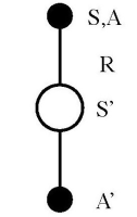
The algorithm used for On-policy TD-control is popularly known as SARSA. The name SARSA, as shown in the figure, indicates a proper sequence of states, actions, and rewards for a time step.
The update equation for SARSA is identical to the one for TD-prediction, except that here we use the action-value function $Q$ instead of the state-value function $V$.
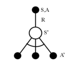
Off-policy TD-Control (Q-learning)
A more straightforward approach towards balancing exploration and exploitation is to use two different policies. A behavior policy $b$ to generate information about the environment and a target policy $\pi$ to evaluate and improve. The former can be used to ensure sufficient exploration and the latter to build a greedy deterministic policy for the agent. We can use techniques like Importance Sampling to use the values from one distribution to generate values for another distribution. However, I won’t go into the details of Importance Sampling in this article.
Q-learning is an off-policy algorithm that can be used for control. Unlike SARSA, in Q-learning, we build an optimal policy by choosing the actions maximizing Q-values, irrespective of the policy being followed, hence making it off-policy.
The update equation for Q-learning is the same as SARSA, except that here we pick the maximum Q-value over all the actions.
Now we see the implementation of both the algorithms and contrast their results.
Setting up the environment
Let us start by defining our environment. We consider the classic problem of Cliff walking. The aim is to safely walk from the Start state $S$ to the Terminal state $T$, avoiding contact with the $x$ states, indicating the cliff. The dimensions of the grid are $4\times12$. The rewards are defined as shown in the code.
Let us write the code for this environment.
'''
#################### CLIFF WALKING ENVIRONMENT #########################

A schematic view of the environment-

            o  o  o  o  o  o  o  o  o  o  o  o
            o  o  o  o  o  o  o  o  o  o  o  o
            o  o  o  o  o  o  o  o  o  o  o  o
            S  x  x  x  x  x  x  x  x  x  x  T

Actions:
    UP (0)
    DOWN (1)
    RIGHT (2)
    LEFT (3)

Rewards:
     0 for going in Terminal state
    -100 for falling in the cliff
    -1 for all other actions in any state

Note: State remains the same on going out of the maze (but -1 reward is given)
      The episode ends and the agent returns to the start state after falling in the cliff

'''
START_STATE = 36
TERMINAL_STATE = 47
def reward(state):
    if(state == TERMINAL_STATE):
        reward = 0
    elif(state > START_STATE and state < TERMINAL_STATE):
        reward = -100
    else:
        reward = -1
    return reward

def env(state, action):
    # return_val = [prob, next state, reward, isdone]
    num_states = rows * columns
    isdone = lambda state: state > START_STATE and state <= TERMINAL_STATE

    if(isdone(state)):
        next_state = state
    else:
        if(action == 0):
            next_state = state - columns if state - columns >= 0 else state
        elif(action == 1):
            next_state = state + columns if state + columns < num_states else state
        elif(action == 2):
            next_state = state + 1 if (state + 1) % columns else state
        elif(action == 3):
            next_state = state - 1 if state % columns else state
    # State Transition Probability is 1 because the environment is deterministic
    return_val = [1, next_state, reward(next_state), isdone(next_state)]
    return return_val
Setting the Hyperparameters
alpha = 0.1 # Learning Rate
epsilon = 0.1 # For Epsilon-greedy policy to balance exploration and exploitation
rows = 4
columns = 12
num_states = rows * columns
num_actions = 4
gamma = 1 # Discount Factor
episodes = 100000 # Number of games played
Code for SARSA
def sarsa():
    # Initialize the action value function
    Q = np.zeros((num_states, num_actions))
    for episode in range(episodes):
        # Initialize S
        curr_state = START_STATE
        # Pick a random number between 0 and 1
        P = np.random.random()
        if(P > epsilon):
            # Pick the greedy action
            curr_action = np.argmax(Q[curr_state])
        else:
            # Pick a random action to explore
            curr_action = np.random.randint(0, num_actions)
        while True:
            # prob: State Transition Probability
            # reward, next_state: Immediate reward and next state on taking curr_action in curr_state
            # isdone: Whether the next state is Terminal or not
            prob, next_state, reward, isdone = env(curr_state, curr_action)
            # Pick a random number between 0 and 1
            P = np.random.random()
            if(P > epsilon):
                # Pick the greedy action
                next_action = np.argmax(Q[next_state])
            else:
                # Pick a random action to explore
                next_action = np.random.randint(0, num_actions)
            # Update the current state-action value
            Q[curr_state, curr_action] += alpha * (reward + gamma * Q[next_state, next_action] - Q[curr_state, curr_action])
            curr_state = next_state
            curr_action = next_action
            if isdone:
                break
    return Q
Analyzing the output of SARSA
#Value Function for SARSA:
 [[ -15.74555335  -17.00770557  -14.72761086  -15.87903553]
  [ -14.80882017  -15.83193455  -13.53643952  -16.1710938 ]
  [ -13.60100703  -14.69401378  -12.31706667  -14.891688  ]
  [ -12.51053159  -13.18760376  -11.07558215  -13.92747595]
  [ -11.26885281  -11.0281459    -9.98001468  -12.65549474]
  [ -10.18428061   -9.68183632   -8.9420201   -11.46398501]
  [  -8.96331482   -8.79880919   -7.80699274  -10.346947  ]
  [  -8.00042743   -8.08516589   -6.69941586   -9.10158426]
  [  -6.77630856   -6.36751754   -5.6489623    -8.18475937]
  [  -5.90454593   -5.30837411   -4.62889594   -6.98658268]
  [  -4.54974112   -4.28644813   -3.37350562   -5.87034597]
  [  -3.68413676   -2.21718067   -3.67062166   -4.77129636]
  [ -15.9003115   -18.24574918  -16.04084254  -17.1047113 ]
  [ -14.72267411  -22.59062716  -15.23052615  -16.87942897]
  [ -14.06782408  -21.64533154  -13.80416604  -15.84413179]
  [ -12.63071163  -21.74775622  -11.1704168   -14.68441167]
  [ -11.4018752   -19.51144135  -10.02965672  -13.33096277]
  [ -10.21018076  -13.57074914   -9.10236663  -11.94916815]
  [  -9.15510096  -17.89348385   -7.87940067  -10.46902327]
  [  -7.95524946  -17.67743594   -6.18437559   -8.58969456]
  [  -6.93863389   -7.61836647   -4.86422572   -7.61089901]
  [  -5.70013343   -8.99483878   -3.55557597   -6.10316268]
  [  -4.6420972    -8.79458691   -2.32539884   -4.88959371]
  [  -3.72007602   -1.46509645   -2.69312713   -3.80690379]
  [ -16.90360883  -24.96096208  -18.63977914  -18.63050672]
  [ -15.94321396  -99.9999088   -16.78022889  -17.63360538]
  [ -14.5763593   -98.17519964  -15.36984983  -20.17387662]
  [ -13.27361553  -96.90968456  -14.0056585   -14.87858063]
  [ -11.9122529   -97.74716005  -14.97223822  -13.31833765]
  [ -10.05614692  -89.05810109  -18.29711103  -11.77550304]
  [  -8.30209779  -91.13706188  -12.78722358  -11.83562135]
  [  -7.87842282  -97.4968445   -19.53350069  -13.83536481]
  [  -6.39617766  -91.13706188  -23.43855218  -10.54015816]
  [  -4.89517746  -97.21871611   -9.83336951   -8.10037857]
  [  -3.79821519  -99.99987489   -1.02922244   -9.71262291]
  [  -2.81170253    0.           -1.40829322   -5.99237393]
  [ -17.8845159   -19.2633337  -100.          -26.75662092]
  [   0.            0.            0.            0.        ]
  [   0.            0.            0.            0.        ]
  [   0.            0.            0.            0.        ]
  [   0.            0.            0.            0.        ]
  [   0.            0.            0.            0.        ]
  [   0.            0.            0.            0.        ]
  [   0.            0.            0.            0.        ]
  [   0.            0.            0.            0.        ]
  [   0.            0.            0.            0.        ]
  [   0.            0.            0.            0.        ]
  [   0.            0.            0.            0.        ]]

# Deterministic Policy obtained from the value function:
 [[2 2 2 2 2 2 2 2 2 2 2 1]
  [0 0 2 2 2 2 2 2 2 2 2 1]
  [0 0 0 0 0 0 0 0 0 0 2 1]
  [0 0 0 0 0 0 0 0 0 0 0 0]]

# map_dict = {0:'UP', 1:'DOWN', 2:'RIGHT', 3:'LEFT'}
The policy obtained after running SARSA chooses a path that starts from $S$ and goes all the way to the top left corner and then takes a right to travel to the top right corner and then goes down to $T$. The net reward for this trajectory is -16 units.
Code for Q-learning
def qlearning():
    # Initialize the action value function
    Q = np.zeros((num_states, num_actions))
    for episode in range(episodes):
        # Initialize S
        curr_state = START_STATE
        while True:
            # Generate a random number between 0 and 1
            P = np.random.random()
            if(P > epsilon):
                # Pick the greedy action
                curr_action = np.argmax(Q[curr_state])
            else:
                # Pick a random action to explore
                curr_action = np.random.randint(0, num_actions)
            # prob: State Transition Probability
            # reward, next_state: Immediate reward and next state on taking curr_action in curr_state
            # isdone: Whether the next state is Terminal or not
            prob, next_state, reward, isdone = env(curr_state, curr_action)
            # Update the current state-action value
            Q[curr_state, curr_action] += alpha * (reward + gamma * np.max(Q[next_state]) - Q[curr_state, curr_action])
            curr_state = next_state
            if isdone:
                break
    return Q
Analyzing the output of Q-learning
# Value Function for Q-learning:
 [[ -13.039192    -12.9009192   -12.90113516  -13.08968947]
  [ -12.14546553  -11.98726119  -11.98725272  -12.13658996]
  [ -11.25291246  -10.99493178  -10.99507023  -11.23775119]
  [ -10.03039412   -9.99773237   -9.99754541  -10.58096787]
  [  -9.41628088   -8.99894028   -8.99886259   -9.77942658]
  [  -8.29639634   -7.99951773   -7.99952633   -8.46326847]
  [  -7.45221489   -6.99978286   -6.99978826   -8.11692331]
  [  -6.51413953   -5.99989923   -5.99989745   -7.48278992]
  [  -5.27000923   -4.99994998   -4.99995151   -6.1610402 ]
  [  -4.25821767   -3.99998262   -3.99998116   -5.06747694]
  [  -3.63427036   -2.99999499   -2.99999524   -4.32412406]
  [  -2.46854951   -2.           -2.3962636    -2.91742446]
  [ -13.81798407  -12.          -12.          -12.99881052]
  [ -12.97399158  -11.          -11.          -12.999805  ]
  [ -11.9823411   -10.          -10.          -11.99946835]
  [ -10.9886305    -9.           -9.          -10.99991042]
  [  -9.99234213   -8.           -8.           -9.99944043]
  [  -8.99620325   -7.           -7.           -8.99978128]
  [  -7.99812993   -6.           -6.           -7.99561701]
  [  -6.99882436   -5.           -5.           -6.99554636]
  [  -5.99767696   -4.           -4.           -5.99955904]
  [  -4.99749209   -3.           -3.           -4.99954533]
  [  -3.99737988   -2.           -2.           -3.99923482]
  [  -2.9986046    -1.           -1.99953839   -2.99821254]
  [ -13.          -13.          -11.          -12.        ]
  [ -12.         -100.          -10.          -12.        ]
  [ -11.         -100.           -9.          -11.        ]
  [ -10.         -100.           -8.          -10.        ]
  [  -9.         -100.           -7.           -9.        ]
  [  -8.         -100.           -6.           -8.        ]
  [  -7.         -100.           -5.           -7.        ]
  [  -6.         -100.           -4.           -6.        ]
  [  -5.         -100.           -3.           -5.        ]
  [  -4.         -100.           -2.           -4.        ]
  [  -3.         -100.           -1.           -3.        ]
  [  -2.            0.           -1.           -2.        ]
  [ -12.          -13.         -100.          -13.        ]
  [   0.            0.            0.            0.        ]
  [   0.            0.            0.            0.        ]
  [   0.            0.            0.            0.        ]
  [   0.            0.            0.            0.        ]
  [   0.            0.            0.            0.        ]
  [   0.            0.            0.            0.        ]
  [   0.            0.            0.            0.        ]
  [   0.            0.            0.            0.        ]
  [   0.            0.            0.            0.        ]
  [   0.            0.            0.            0.        ]
  [   0.            0.            0.            0.        ]]


# Deterministic Policy obtained from the value function:
 [[1 2 1 2 2 1 1 2 1 2 1 1]
  [1 1 1 1 1 1 1 1 1 1 1 1]
  [2 2 2 2 2 2 2 2 2 2 2 1]
  [0 0 0 0 0 0 0 0 0 0 0 0]]

# map_dict = {0:'UP', 1:'DOWN', 2:'RIGHT', 3:'LEFT'}
The policy obtained after running Q-learning chooses a path that starts from $S$ and takes a right just after moving one step up from $S$, all the way to the right, and then moves one step down to reach $T$. The net reward for this trajectory is -12 units.
Comparing the two outputs
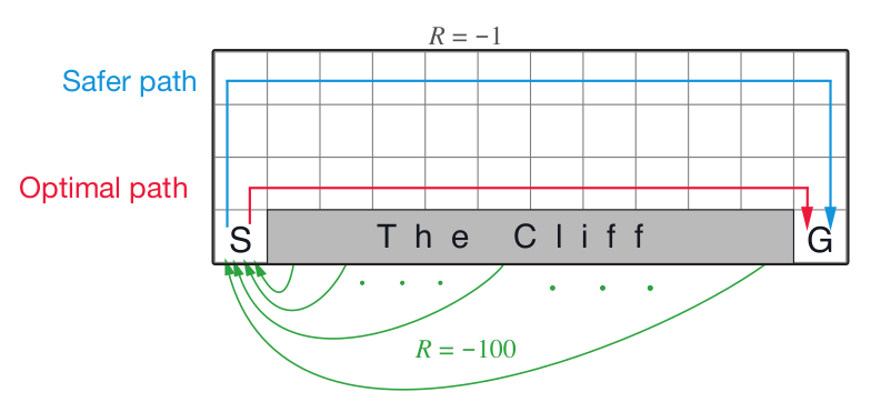
An important thing to notice in the two outputs is the path that the two algorithms find after playing the game for 10000 trials. The output reflects the conservative nature of SARSA as it finds a safer path to the terminal state. Here “safer” means that the trajectory is at a good enough distance from the cliff, and there is less chance that the agent could wall into it. However, the path earns a net reward of -16 units, which is less than one with Q-learning.
In contrast to this, we see that Q-learning finds the Optimal path to $T$, which goes just over the cliff. Hence we get the maximum possible reward -12 units on following this policy. However, this path is a bit unsafe because there is more probability that the agent could fall into the cliff while training.
But why did this difference come up?
The answer lies in the nature of the two algorithms. One is on-policy, and the other is off-policy. Recall that off-policy finds the optimal policy, while on-policy converges to a near-optimal policy (results of on-policy may differ on tuning the hyperparameters). In both the algorithms, we “take” an action according to $\epsilon$-greedy policy, but in Q-learning, we use the maximizing action, irrespective of the action “taken”. However, SARSA uses the same action to make updates. This means that SARSA pays for the exploratory moves it makes using a near-optimal policy that still explores. This makes SARSA more conservative.
Following this, in the cases where the optimal moves are close to highly negative rewards, SARSA tends to avoid an optimal but dangerous path. If we change the negative reward for falling off the cliff to -50 units or even lower (in magnitude), then SARSA takes a less safe path, which goes closer to the cliff. This indicates that as we make the magnitude of the negative reward higher, SARSA tends to be more conservative.
Although Q-learning finds the optimal policy, its online performance is worse than SARSA (because of the closeness between the path and the cliff) in this case where we have set $\epsilon$ = 0.1. If we choose a lower exploration rate like 0.01, then Q-learning does better. Nevertheless, asymptotically, both converge to the optimal policy if $\epsilon$ is decreased over time.
Expected SARSA
Let us consider an update rule just like Q-learning, but with an Expectation over all the state-action pairs instead of a maximum. This algorithm is known as Expected SARSA.
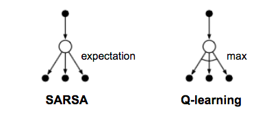
We can use it both on as well as off-policy. If $\pi$ is a greedy policy while the behavior being exploratory, then Expected SARSA is exactly Q-learning. Hence this generalizes Q-learning and improves considerably over SARSA. Having these properties, Expected SARSA may outperform both SARSA and Q-learning with some additional computational cost.
Conclusion
In this article, we saw some well-known methods to solve Reinforcement Learning problems using bootstrapping and sampling. However, it is difficult to extend these algorithms to real-world RL problems. Real-world RL problems like the game of Go can have up to $10^{170}$ states and more than $200$ possible moves to make at a time, and many problems like teaching a Helicopter to fly in a park, a robot trying to manipulate objects, etc. can have extremely large or asymptotically infinite state and action spaces. The table-lookup representation used until now is highly impractical to solve these problems. Hence we use function approximators like Neural-Networks to find an approximate action-value function rather than finding the value for each state-action pair. In a nutshell, the approximator is chosen and tuned such that it can represent the values and probabilities for the whole state-action space in a finite and small number of parameters. However, the core logic behind the algorithms remains the same, just with a change in the way they are implemented.